
In the NBA, understanding a player’s future potential is essential for general managers. Roster decisions affect not just the current season but also a team’s trajectory for years to come. Overcommitting to players on the verge of decline can cripple a team, while signing a player before a breakout can provide a significant boost. In this project, I will simulate NBA player careers based on their current stats to project their future value.
To do this, we need a reliable metric to estimate a player’s impact. Wins Above Replacement (WAR) is an advanced yet interpretable statistic derived from Value Over Replacement Player (VORP) and Box Plus-Minus (BPM). WAR estimates how many wins a player contributes to a replacement-level player, accounting for both per-possession effectiveness and playing time. By normalizing WAR to an 82-game season, we can compare players on a consistent scale, regardless of how many games they’ve played.
With WAR data spanning multiple seasons, we can model the expected year-to-year changes in a player’s WAR and the uncertainty of these predictions. Using this model, I will simulate the careers of current NBA players to forecase their potential performance in the coming years.
Data
To build the dataset for this project, I webscraped advanced player stats from Basketball Reference for every season since 1990. This site provides key information, including each player’s playing time and Value Over Replacement Player (VORP). While VORP can be difficult to interpret on its own, it can easily be converted to WAR by multiplying VORP by 2.7, as suggested by Basketball Reference. I then adjusted these WAR values to an 82-game season to create a consistent WAR per 82 games (WAR/82) metric. Next, I filtered the data to include only players who participated in at least 25 games in two consecutive seasons since the goal is to predict year-to-year changes in WAR. After these steps, the dataset comprised of 8601 samples.
Wins Above Replacement
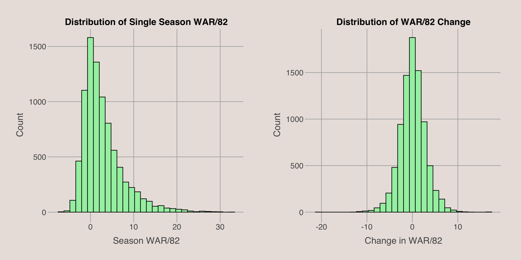
To begin, let’s examine the distribution of WAR per 82 games. The plots below show the distribution of WAR/82 for a single season and the distribution of the change in WAR/82 from one season to the next among qualifying players. The WAR/82 distribution is right-skewed, reflecting the fact that All-Star level players have a much larger impact on their team’s success than others. The distribution of the change in WAR/82 is roughly symmetric around 0, indicating that, on average, players tend to maintain their performance from year to year, with an equal likelihood of improving or declining if no other factors are considered. Typically, the change in WAR/82 from season to season falls between -5 and +5.
To gain deeper insights, we can analyze the change in WAR/82 by conditioning on other variables. One such variable is a player’s performance in the previous season. By binning the previous season’s WAR/82 into categories, we can explore how changes in WAR/82 depend on recent performance. I categorized previous WAR/82 into six groups: negative impact (WAR/82 below 0), minimal impact (WAR/82 between 0 and 2.5), bench (WAR/82 between 2.5 and 5), starter (WAR/82 between 5 and 10), All-Star level (WAR/82 between 10 and 15), and All-NBA level (WAR/82 over 15). While these cutoffs are somewhat arbitrary, they effectively convey the concept.
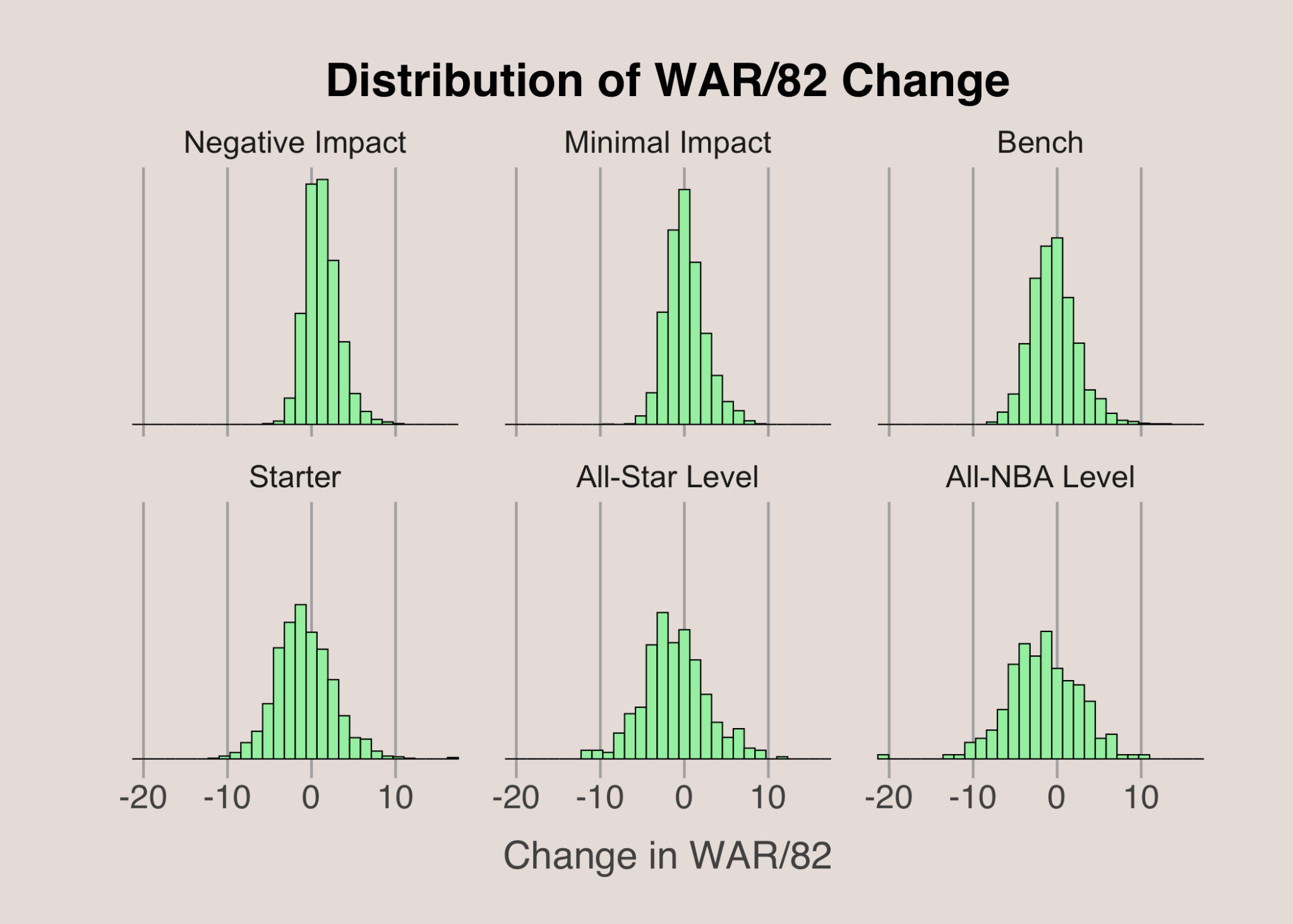
The visual above demonstrates that a player’s most recent performance does influence the distribution of changes in WAR/82. Although the center of each distribution is close to 0, the spread varies significantly. Higher-performing players tend to experience more significant fluctuations in WAR/82, while less impactful players exhibit smaller changes. Additionally, the variability in WAR/82 changes is influenced by the player’s draft position.
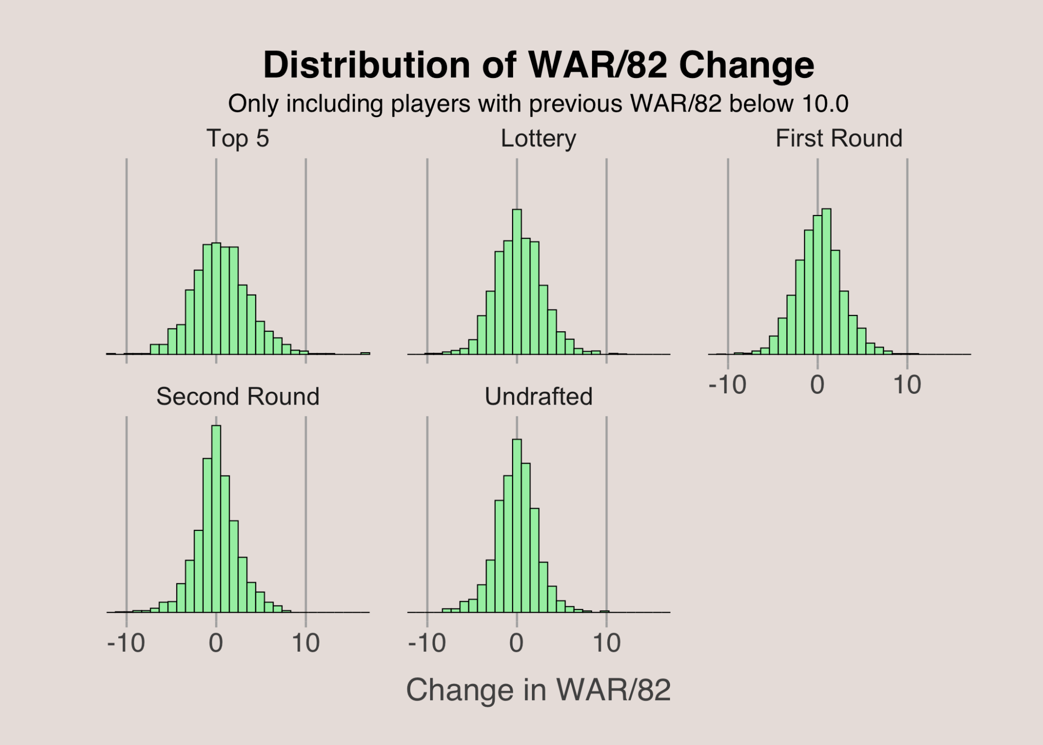
When examining the change in WAR/82 based on draft pick, we again observe differences in the distribution’s variability. This visual excludes players with a previous season WAR/82 above 10, as higher draft picks are more likely to be top performers, and we’ve already seen that top performers experience greater variability in WAR/82 changes. Even with these exclusions, top 5 picks tend to show more significant fluctuations in WAR/82, while later picks exhibit less variability. This suggests that higher draft picks are more prone to substantial improvements or declines than second-round picks or undrafted players.
A key takeaway from this exploratory data analysis is that the variance in changes in WAR/82 is not constant. This is crucial for modeling because ordinary least squares, the most commonly used regression model, assumes constant variance—a condition that doesn’t seem to hold here. Therefore, a more flexible model that can accommodate varying variances across samples will likely be necessary.
Modeling
Features
To begin modeling, we need to define our response variable—the change in WAR/82 from season to season—and identify the features that will help us predict it. Key features include a player’s age and draft pick, as these are strong indicators of future performance. Additionally, I incorporated other relevant features to provide a fuller picture of a player’s career trajectory and current performance. The final set of features includes the player’s previous season’s WAR/82, career WAR/82, most recent change in WAR/82, and a weighted change in WAR/82. These features offer insight into a player’s career progression and how their performance may evolve.
Here are the six main features used to predict the change in WAR/82 from the prior season to the upcoming season:
- Age: The player’s age at the start of the upcoming season
- Career WAR/82: The player’s cumulative WAR/82 up to the current point in their career
- Log Pick: The logarithm of the player’s draft pick (with undrafted players assigned a pick value of 80)
- Previous Change: the change in WAR/82 from two seasons ago to the prior season
- Previous WAR/82: The player’s WAR/82 in the prior season
- Weighted Change: The exponentially weighted average change in WAR/82 across a player’s career, with more recent changes weighted more heavily. The most recent change is weighted twice as much as the next most recent change, and so on.
The weighted change is calculated using the following formula:
- WC: Weighted change for a given season
- s: Prior season
- d: Rookie season
- WARk: WAR/82 in season k
- gk: number of games played in season k
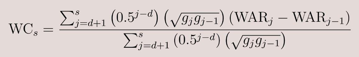
This formula takes into account a player’s change in WAR/82 across all consecutive seasons in their career, emphasizing more recent changes to better capture current performance trends.
Ordinary Least Squares
The most common model for predicting outcomes is Ordinary Least Squares (OLS). The OLS model follows this form:
In this model, each prediction (yi) is assumed to follow a normal distribution, where the mean is a linear combination of the features (xi) and their corresponding coefficient (![]() ), while the variance remains constant across all samples. A key assumption in OLS is that this variance is fixed for all observations. To check if this assumption holds, I examined the residuals—the differences between the actual values and the predicted values. If there are discernible patterns in the residuals, it suggests that the fixed variance assumption is violated.
), while the variance remains constant across all samples. A key assumption in OLS is that this variance is fixed for all observations. To check if this assumption holds, I examined the residuals—the differences between the actual values and the predicted values. If there are discernible patterns in the residuals, it suggests that the fixed variance assumption is violated.
I fit an OLS model using the six feature variables described earlier, with the change in WAR/82 as the response variable. To assess whether the fixed variance condition is met, I examined the relationship between the residuals and one of the feature variables—the previous season’s WAR/82. The plots below reveal a clear pattern: players with higher WAR/82 in the prior season exhibit greater variance in their residuals, while lower-impact players have smaller residual variance. This indicates that the fixed variance assumption is indeed violated. As a result, we need to explore alternate models that can accommodate varying variances for each sample.
Bayesian Model Averaging
An alternative modeling approach is Bayesian Model Averaging (BMA). In BMA, we first specify the sampling model and set priors for all parameters. We then run an algorithm to obtain the posterior distributions for each parameter. One of the strengths of Bayesian modeling is the ability to allow each coefficient to be turned on or off, which helps prevent overfitting by avoiding the inclusion of too many parameters.
In the Bayesian model averaging approach, I included both linear and second-order terms as features. The linear terms are the same six features used in the OLS model. The second-order terms consist of squared versions of the linear terms as well as interaction terms between all pairs of features.
After preparing the data and creating the second-order terms, I standardized all the features and the response variable to ensure everything is on the same scale. This standardization simplifies the process or running the algorithm and obtaining posterior distributions for the parameters.
Sampling Model
To specify the sampling model, we need to define how the data is generated. Here is the mathematical representation of the sampling model I used:
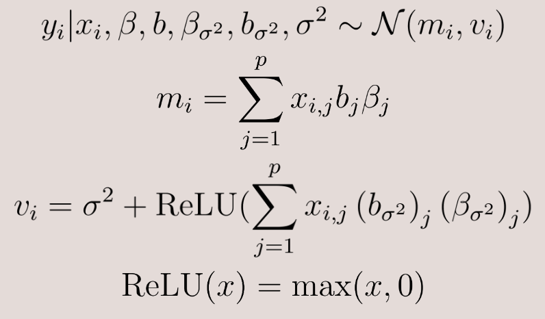
We can break this down:
- Distribution of yi: Each response, which is the change in WAR/82, is assumed to come from a normal distribution with mean mi and variance vi
- Mean (mi): The mean is calculated as a linear combination of the feature vector (xi), the coefficient vector (
 ), and a binary vector (b). The feature vector and coefficient vectors are similar to those in the OLS model, with the addition of second-order terms and their corresponding coefficients. The binary vector (b) contains 0’s and 1’s to indicate whether each coefficient is active, helping to prevent overfitting by selectively including features
 - Variance (vi): The variance consists of a constant term (
 ) plus a sample-specific term. The sample-specific term is derived from a linear combination of the feature vector, a different coefficient vector, and a different binary vector. This term accounts for additional variance specific to each sample beyond the baseline variance. The ReLU function ensures that this additional variance is non-negative, avoiding the possibility of a negative variance, which is not feasible. This setup also makes sigma squared interpretable as the baseline or minimum variance.
Priors
For Bayesian Model Averaging, we need to specify priors for each parameter. These priors represent our initial beliefs before observing any data.
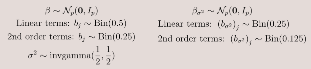
- Coefficient Vectors: For both coefficient () vectors, I used normal priors. Each element in these vectors is assigned a normal distribution with a mean of 0 and a standard deviation of 11. Since the features are standardized, this is appropriate.
- Binary Vectors for Mean: For the binary vector associated with the mean, each element has a prior probability of being included as follows. This means that second-order terms (squared terms and interaction terms) are less likely to be included, promoting a simpler model.
- Linear terms: Probability of 50%
- Second-order terms: Probability of 25%
- Binary Vectors for Variance: For the binary vector associated with the variance, the prior probabilities are below. The lower prior probabilities indicate that the coefficients affecting variance must show stronger evidence to be included in the model compared to those affecting the mean.
- Linear terms: Probability of 25%
- Second-order terms: Probability of 12.5%
- Baseline variance: The prior for the baseline variance () follows an inverse gamma distribution. This choice ensures that the variance is always positive, as variance cannot be negative.
Markov Chain Monte Carlo
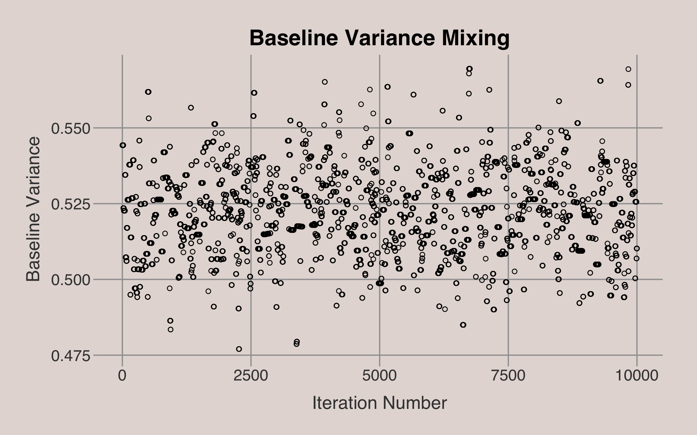
Once we have specified the sampling model and priors, the Metropolis-Hastings algorithm can be used to estimate the posterior distribution. This algorithm approximates the posterior distribution by simulating plausible values for each parameter through many iterations. In my implementation, I discarded the first 100 samples to allow the chain to converge and then ran the algorithm for 10,000 iterations. The results of this simulate are detailed in the “Results” section of this article.
To illustrate, consider how the algorithm simulates the posterior distribution for the baseline variance2. After discarding the initial 100 samples, the algorithm iteratively proposes new values for the baseline variance. At each step, a new value is proposed based on a proposal distribution derived from the current value. We then decide whether to accept the proposed value or retain the current value based on the ratio of the posterior probabilities.
For instance, if the current baseline variance is 0.5, a proposed new value might be 0.51. We calculate the posterior probabilities of the parameters given both the current and proposed values of the baseline variance. By comparing these probabilities, one can determine whether to accept the proposed value or stick with the current one3. The entire chain of baseline variance values4 over the 10,000 iterations is shown in the plot below.
Model Performance Comparison
To evaluate and compare the performance of the Ordinary Least Squares (OLS) model and the Bayesian Model Averaging (BMA) approach, I used two metrics: root mean squared error (RMSE) and mean log likelihood. Instead of comparing raw values, I assessed each model’s performance relative to a baseline model5 that predicts every sample using the mean of the response variable. The comparison results are shown in the plot below. A higher bar indicates better model performance for both metrics.
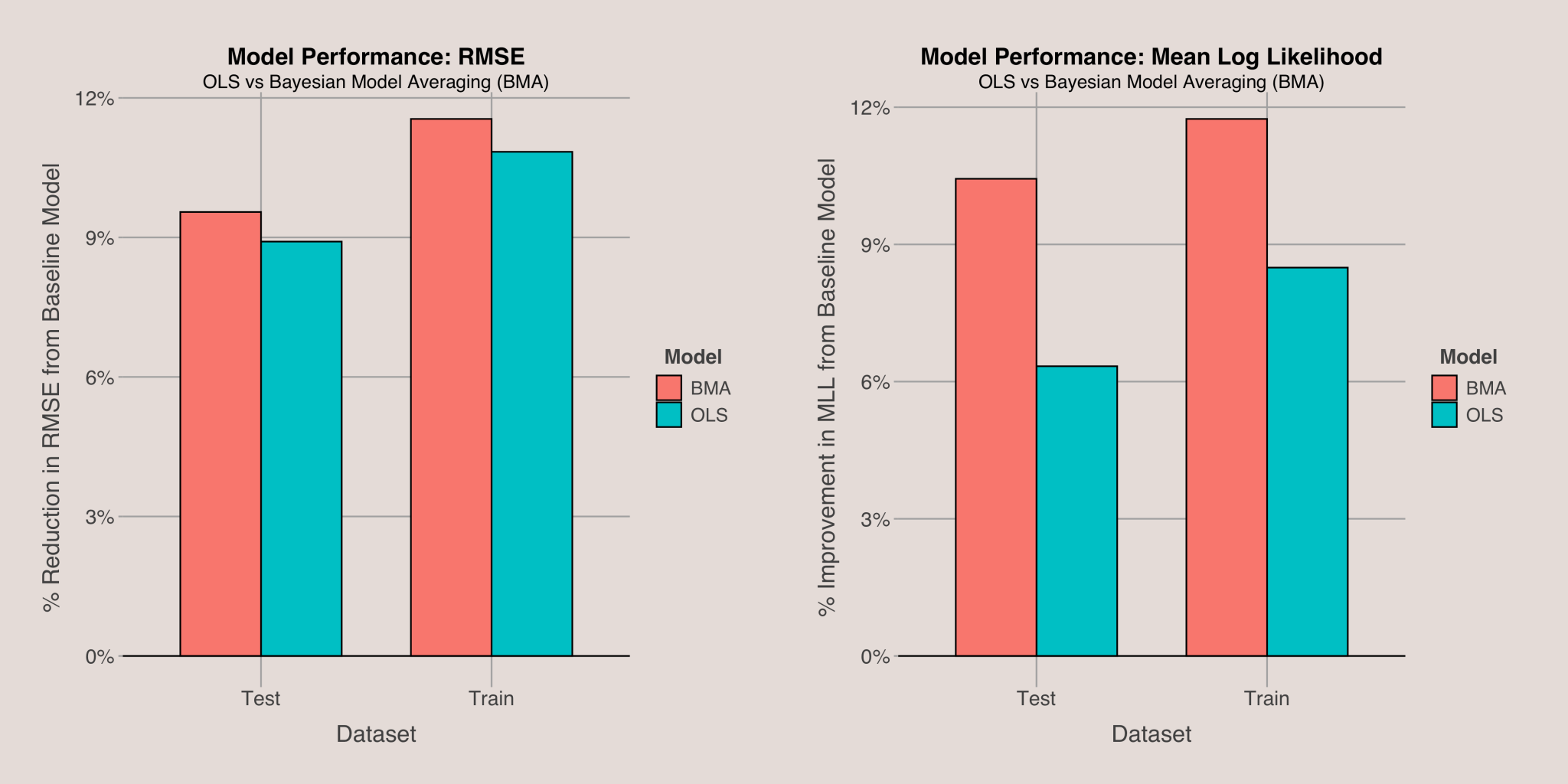
The Bayesian Model Averaging approach outperforms the OLS model in both RMSE and mean log likelihood. Notably, BMA shows significant improvement in log likelihood, which aligns with its design to accommodate flexible variance. Unlike RMSE, which does not account for prediction variance, mean log likelihood considers it, making BMA’s advantage in this metric logical. Specifically, BMA achieved about 1.5 times better performance in terms of the percentage improvement in mean log likelihood compared to OLS. This demonstrates that BMA provides a superior model fit compared to OLS in this context.
Results
Having established that the Bayesian Model Averaging approach outperforms Ordinary Least Squares, we can now examine the BMA results to identify key features driving predictions.
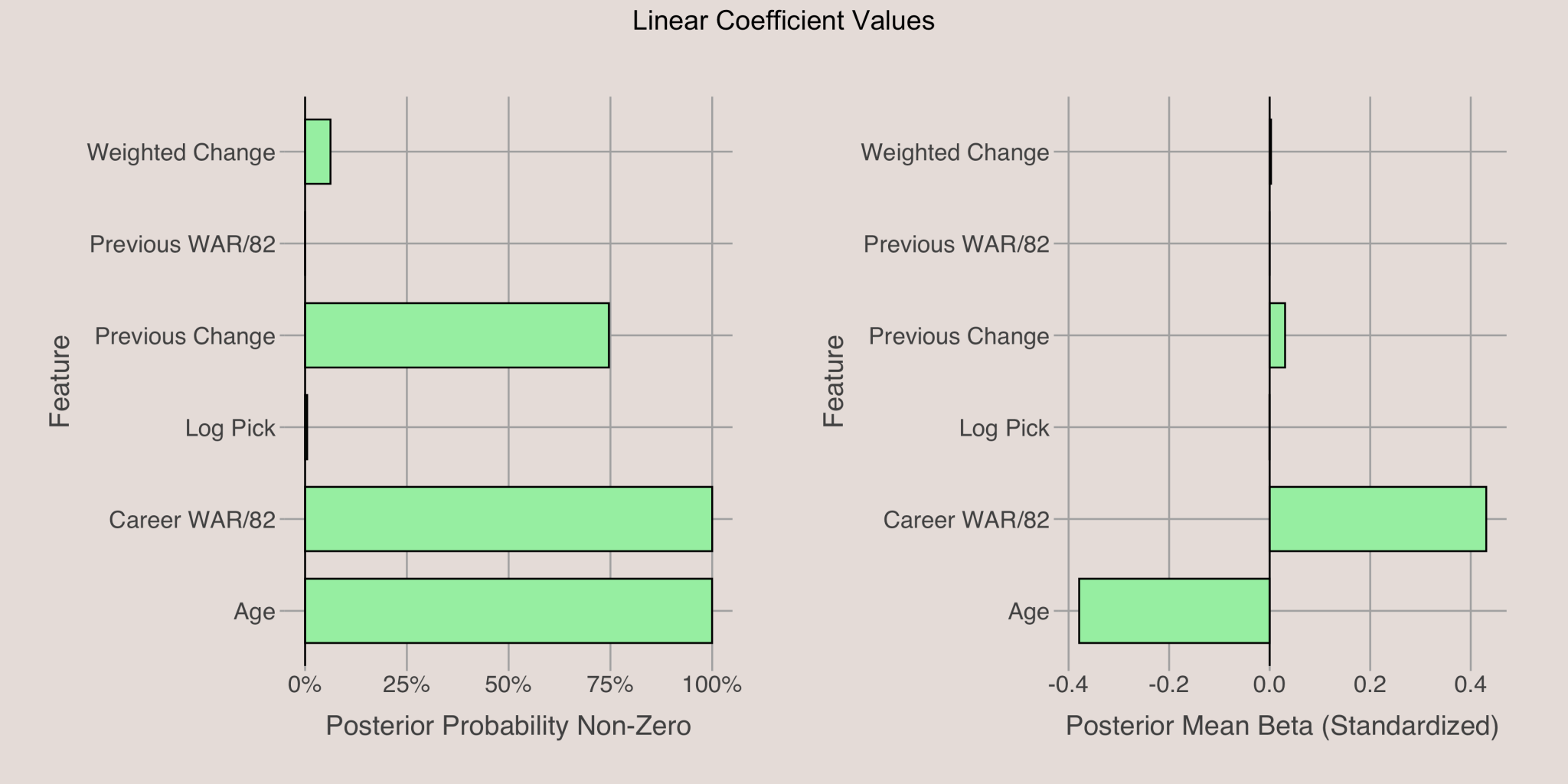
Linear Coefficents
The plot below shows the posterior probabilities6 and mean values of linear coefficients for the response variable. The most influential features are age and career WAR/82, with previous change in WAR/82 also having a small effect. The other linear features have a negligible impact. Specifically, younger players and those with higher career WAR/82 are more likely to show improvement.
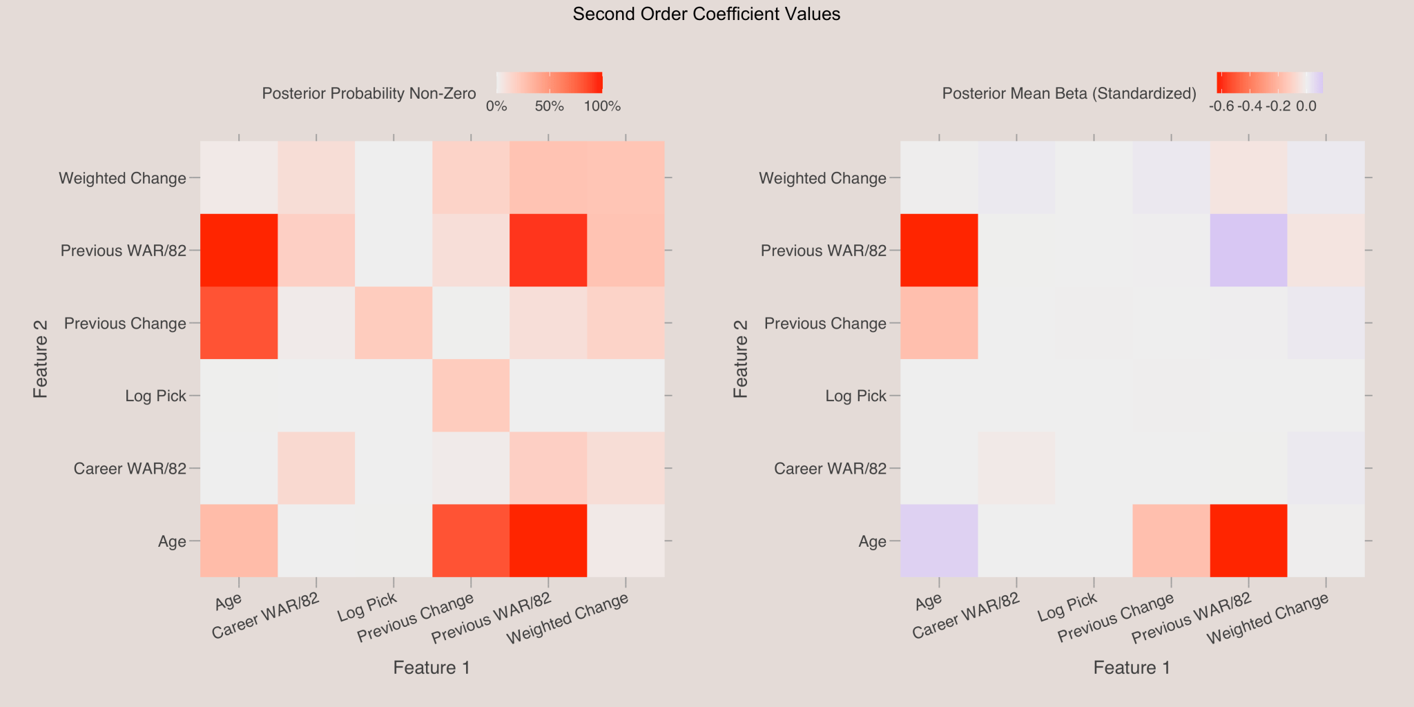
2nd Order Coefficients
The heatmap below displays the posterior probabilities and mean values for the 2nd order coefficients. Each cell represents the effect of interactions between features. Notably, the interaction between previous WAR/82 and age is significant. The negative coefficient indicates that younger players with a high prior season WAR/82 are more likely to see significant improvement, suggesting that young, high-performing players have the potential to become superstars.
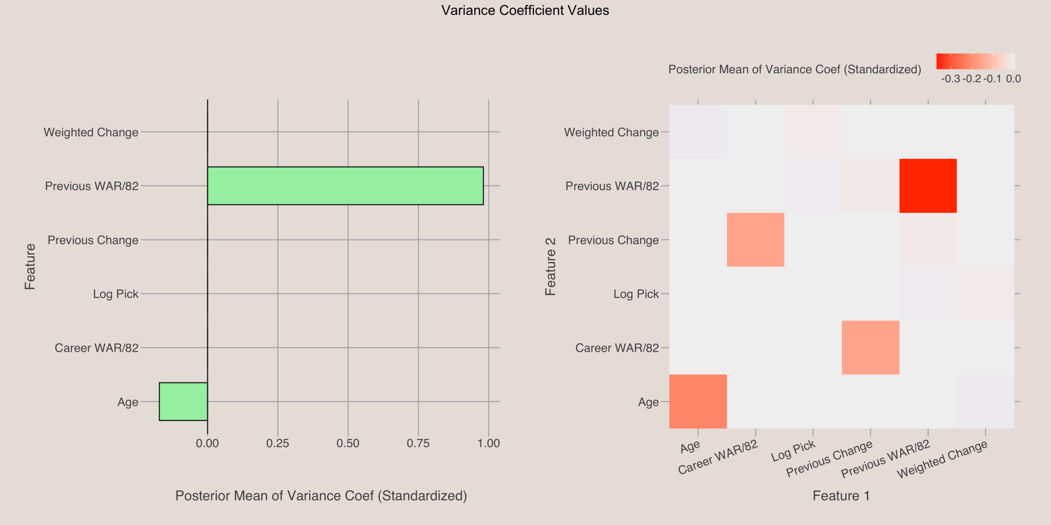
Variance Coefficients
The plot below shows the posterior means for the variance coefficients. The previous season’s WAR/82 is crucial, as indicated by a coefficient with a large magnitude. The positive coefficient for this variable means players with high WAR/82 have more variable future performance. Conversely, a slightly negative coefficient for age suggests that younger players experience more variance in their performance.
Aging Curve
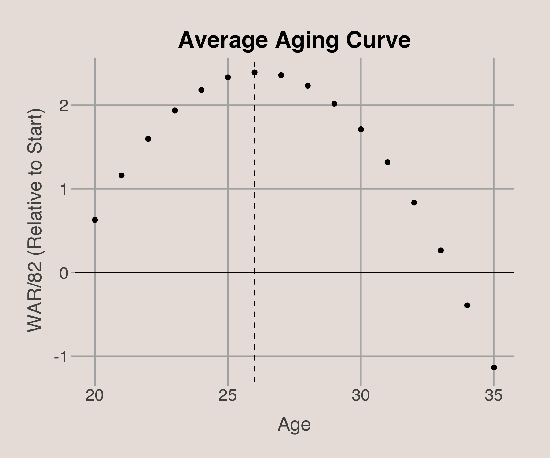
Using the posterior mean coefficients, we can construct an “average” aging curve for NBA players. This curve illustrates the typical progression of a player’s career, peaking around age 26, with the prime years spanning from ages 24 to 29.
Simulating Careers
With our model predicting the distribution of changes in a player’s WAR/82 from season to season, we can simulate player careers. By using current feature values, generating WAR/82 change distributions, and updating features each season, we can simulate multiple career paths and obtain a distribution of future performances.
To summarize a player’s career, I used the average WAR/82 over their best 5-year stretch. This provides a single number representing their performance. To interpret these numbers, I categorized players based on WAR/82 into seven groups7:
- Negative Impact: WAR/82 less than 0
- Minimal Impact: WAR/82 between 0 and 2.5
- Bench: WAR/82 between 2.5 and 5
- Starter: WAR/82 between 5 and 10
- All-Star Level: WAR/82 between 10 and 15
- All-NBA Level: WAR/82 between 15 and 20
- MVP Candidate: WAR/82 above 20
For instance, simulating Victor Wembanyama’s career over the next 10 years for 1000 iterations suggests he is very likely to become an All-NBA or MVP caliber player, aligning with fan expectations.
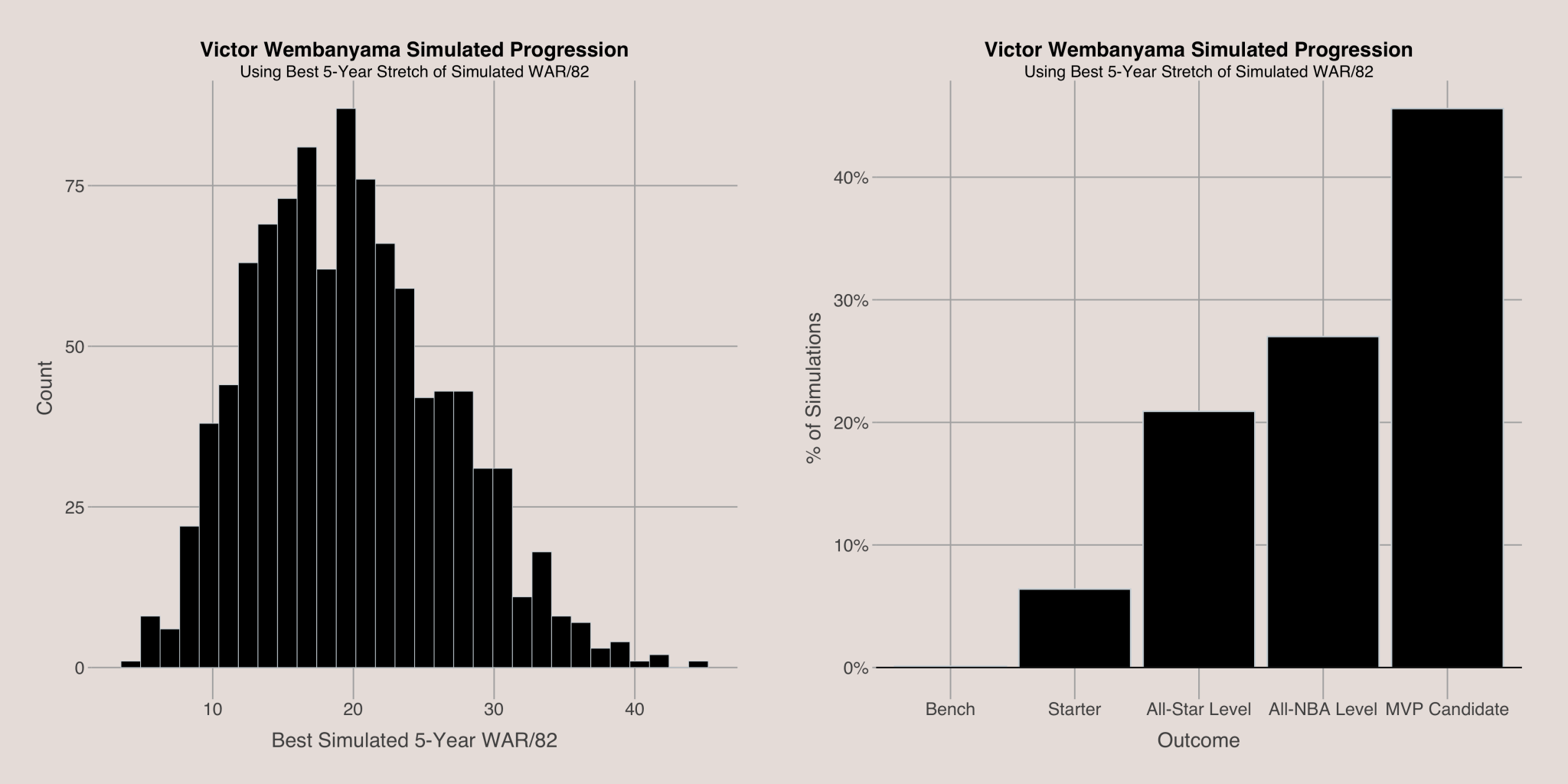

Photo Credit: Scott Wachter-USA TODAY Sports
We can apply this simulation with for all players with sufficient playing time. For example, the future projections for the top picks from 2019 to 2022 reveal Zion Williamson has the best outlook, while Cade Cunningham shows the least likelihood of reaching an All-NBA level or better. Note that these categories are based on WAR/82, which might not always reflect public perceptions. For example, Paolo Banchero’s WAR/82 of 6.37 places him in the “Starter” category, despite his recent All-Star selection. You can simulate any player’s career using this web application: Simulation Tool.
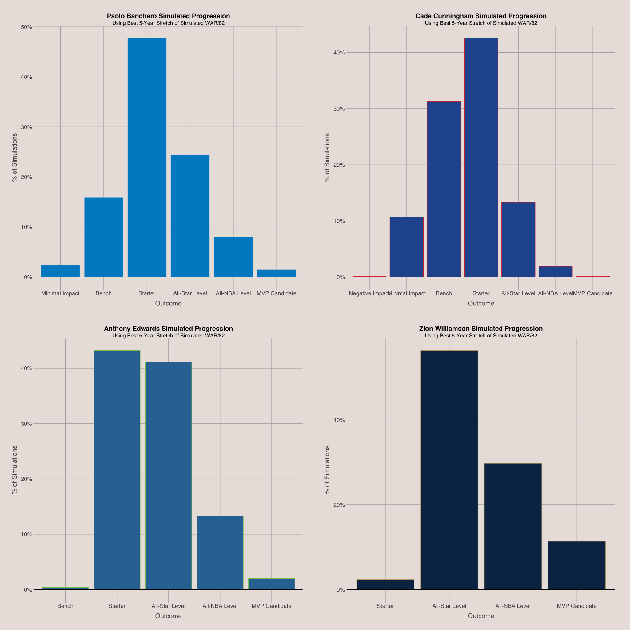

Photo Credit: Britannica
Conclusion
Estimating career progression is crucial for general managers to make strategic decisions that shape their team’s future. By using Bayesian model averaging, we can forecast year-to-year changes in wins above replacement per 82 games (WAR/82) based on historical performance. The model reveals that younger players and those with a strong career track record are more likely to show improvement. Additionally, players with strong previous seasons tend to have higher variance in their WAR/82 changes compared to those with less impact. This approach allows us to simulate player careers and assess the likelihood of achieving All-Star, All-NBA, or MVP status, providing a valuable tool for future player projections.
See the code used to create these visualizations and model here: https://github.com/AyushBatra01/Simulate-Progression
Footnotes:
- The choice of 1 for the prior standard deviation is arbitrary. It is possible that the model could be improved by using cross-validation and trying out different prior standard deviation values on a validation set. However, the MH algorithm took a long time to run, so I did not want to increase the runtime by doing a time-expensive cross-validation analysis. ↩︎
- In the Metropolis-Hastings algorithm, I could not derive the full conditional distribution for the baseline variance parameter. Therefore, I had to use a proposal distribution for simulation. Proposal distributions also had to be used for the variance coefficient parameters. Full conditionals could be derived, and therefore were utilized, for the mean coefficient parameters and all parameters in both binary vectors. ↩︎
- The exact method of choosing to keep the existing value or accept the new one is a stochastic process: we calculate the ratio of the posterior probability using the new value vs the old value, then accept the new value with a probability equal to that ratio (or with probability of 1 if the ratio is greater than 1) ↩︎
- The effective sample size for the baseline variance simulations was about 338, which is unfortunately much lower than the number of iterations (10,000). It is possible this could be improved by trying out different proposal distributions. ↩︎
- The exact method of comparing to the baseline method is as follows: 1) set the baseline model to be the model if we knew nothing about the observation, aka predicting the mean for each sample; 2) calculate the metric for the baseline model; 3) get the % improvement [if want to maximize the metric, like mean log likelihood] or % reduction [if want to minimize the metric, like RMSE] against the baseline model ↩︎
- Posterior probability of the binary vector element for the variable being active ↩︎
- The cutoffs for these groupings are arbitrary ↩︎
