
What is the optimal NBA team—the one that would win the most regular-season games? At first glance, you might think it’s just a lineup of today’s top stars like Shai Gilgeous-Alexander, Nikola Jokic, and Giannis Antetokounmpo. However, the reality of salary caps and luxury tax aprons prevent stacking a roster with max contract superstars. And even if money were no problem, fit is important. Most elite players are high usage shot creators, but a championship-caliber team also needs low-usage specialists who finish plays efficiently and defend at a high level.
This makes team building an optimization problem: choose a limited roster within a fixed budget to maximize expected wins1. Many optimization methods exist, but genetic algorithms are especially well-suited here because they easily incorporate these penalties. They converge toward an optimal solution by simulating evolution, creating an initial pool of candidate rosters then iteratively applying selection, mutation, and crossover. However, before running the algorithm, we need a reliable way to project each player’s future production.
Expected Future Production
When building a team, past performance isn’t enough. Instead, we need to project how players will perform next season. Age, usage rate, and other factors can shift production year to year. Here, production is measured using WAR (wins above replacement) per 82 games, and the goal is to predict each player’s WAR/82 for the following season. To keep things simple, we use just four predictors: the previous year’s WAR/82, age, games played, and usage rate. A linear regression on these variables gives an R² of 0.57. This is solid, though it could be improved with more historical data. However, the main focus here is optimization and not necessarily perfect forecasting, so I stick with this streamlined model. Its predictions form the basis for building the optimal roster for next season.
Fit Penalties
A key part of optimizing NBA teams is accounting for player fit. We want to know how well players’ skills complement each other without too much overlap. Important dimensions of fit include usage, shooting, defense, and passing. To capture these, we use advanced metrics as proxies: usage rate (abbreviated USG%; percentage of offensive plays ending in a shot or turnover), three-point attempt rate (3PAr; share of shots from three), assist rate (AST%; percentage of made field goals assisted while on court), and defensive box plus/minus (DBPM; estimated points prevented per 100 possessions). All variables are standardized to have mean 0 and standard deviation 1 so they’re comparable.
We start by calculating fit penalties for pairs of players. For players A and B, we calculate the penalty with the following formula:

This is similar to a vector dot product, except that for shooting, passing, and defense, I cap positive values at zero before multiplying. The idea is that having multiple good shooters, passers, or defenders isn’t a problem, but having multiple poor ones is. These terms only contribute to the penalty if both players are below average, in which case the product is positive, adding to the penalty.
For example, using 2025 data, the best fitting pair was LaMelo Ball and Jericho Sims as Ball’s high usage and strong shooting and passing paired well with Sims’ low usage and defensive strengths. The worst fit was Zion Williamson and Giannis Antetokounmpo, two high-usage players that limit floor spacing.
To extend this to a full roster, I calculate the penalty for every unique player pair on the team and take the average. This average, when scaled by a user-selected penalty strength parameter2, is the team’s overall fit penalty.
Genetic Algorithm
The core of the project is using a genetic algorithm to assemble the optimal NBA team. A genetic algorithm is an optimization method that mimics evolution to search for the best solution. We begin with a population of random candidate teams, each represented by a binary vector, where 1 means the player is on the roster and 0 means they’re not. Initial teams have 12 randomly chosen players.
Each candidate is evaluated with a fitness function that sums the team’s projected WAR/82 for next season, adjusted for constraints. Any team exceeding 12 players or going over the salary cap gets a fitness score of zero. Candidates are then selected for the next generation, with higher-fitness teams having a greater chance of survival3.
To create new candidates, we choose “parents” from the survivors and perform crossover to combine their traits. Crossover involves swapping segments of the parent vectors at random points. We also introduce mutations by flipping a few random vector entries to keep the search diverse. This process repeats for many generations, ending when we hit a set limit or stop improving the best solution.
The algorithm’s performance depends on tuning parameters such as selection rate, number of parents, crossover points, and mutation probability, which I set based on tests with sample data. While more complex than random search, this method is far more effective. Given the huge number of possible rosters, exhaustive search is impossible, and random guessing is unlikely to find a top team. Genetic algorithms, by contrast, explore the search space in an intelligently, steadily evolving toward high-performing rosters.
Applications
Optimal NBA Team – All Players
Now we can put the genetic algorithm to work. While the method cannot guarantee a truly optimal roster, since checking every possible lineup is computationally impossible, it’s highly likely to find one that’s close.
In this example, we consider all NBA players, limit the roster to 12, and require the total salary to stay under the 2026 luxury tax threshold of $187.9M. The algorithm converged on its best solution after about 150 generations:
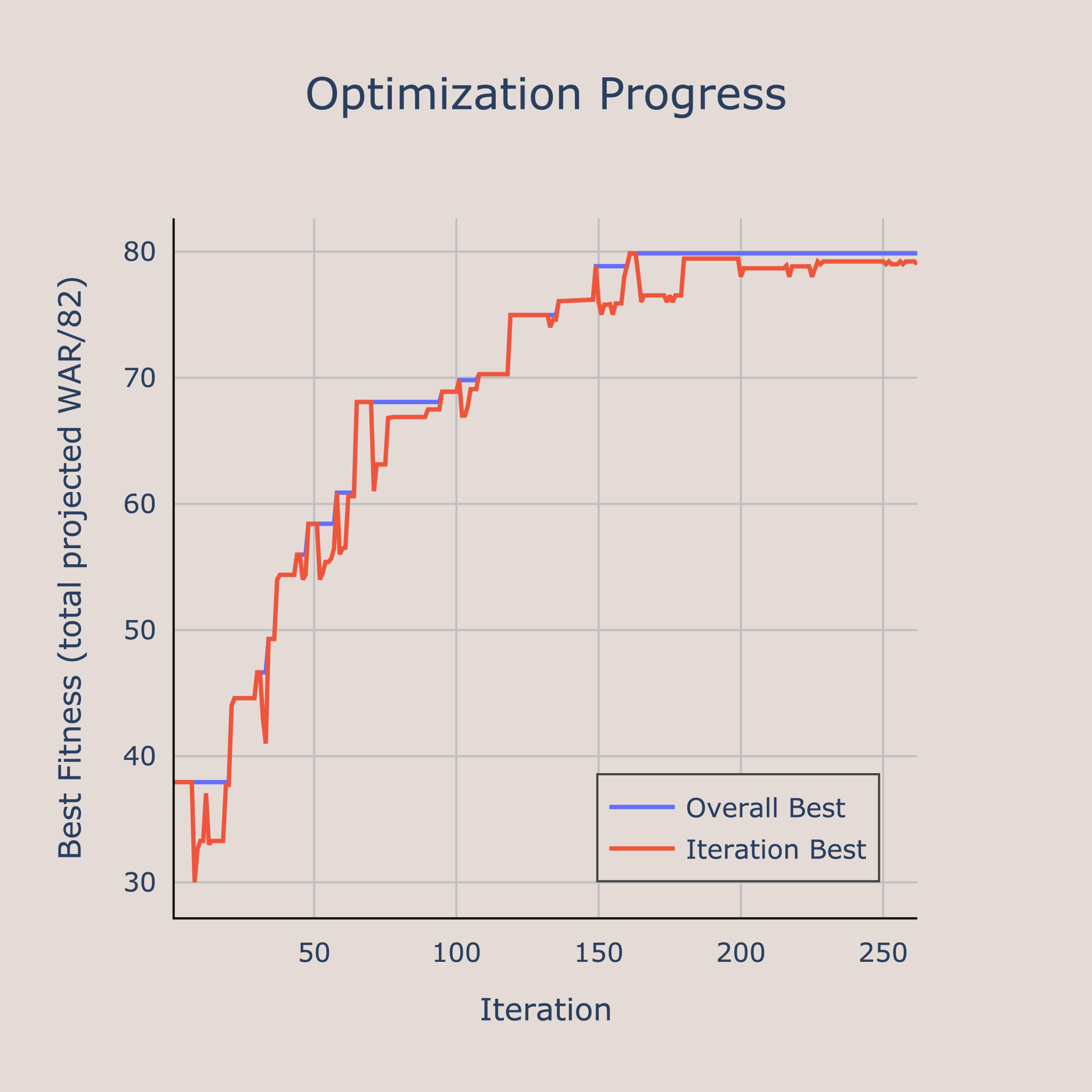
The optimal team found is shown below:

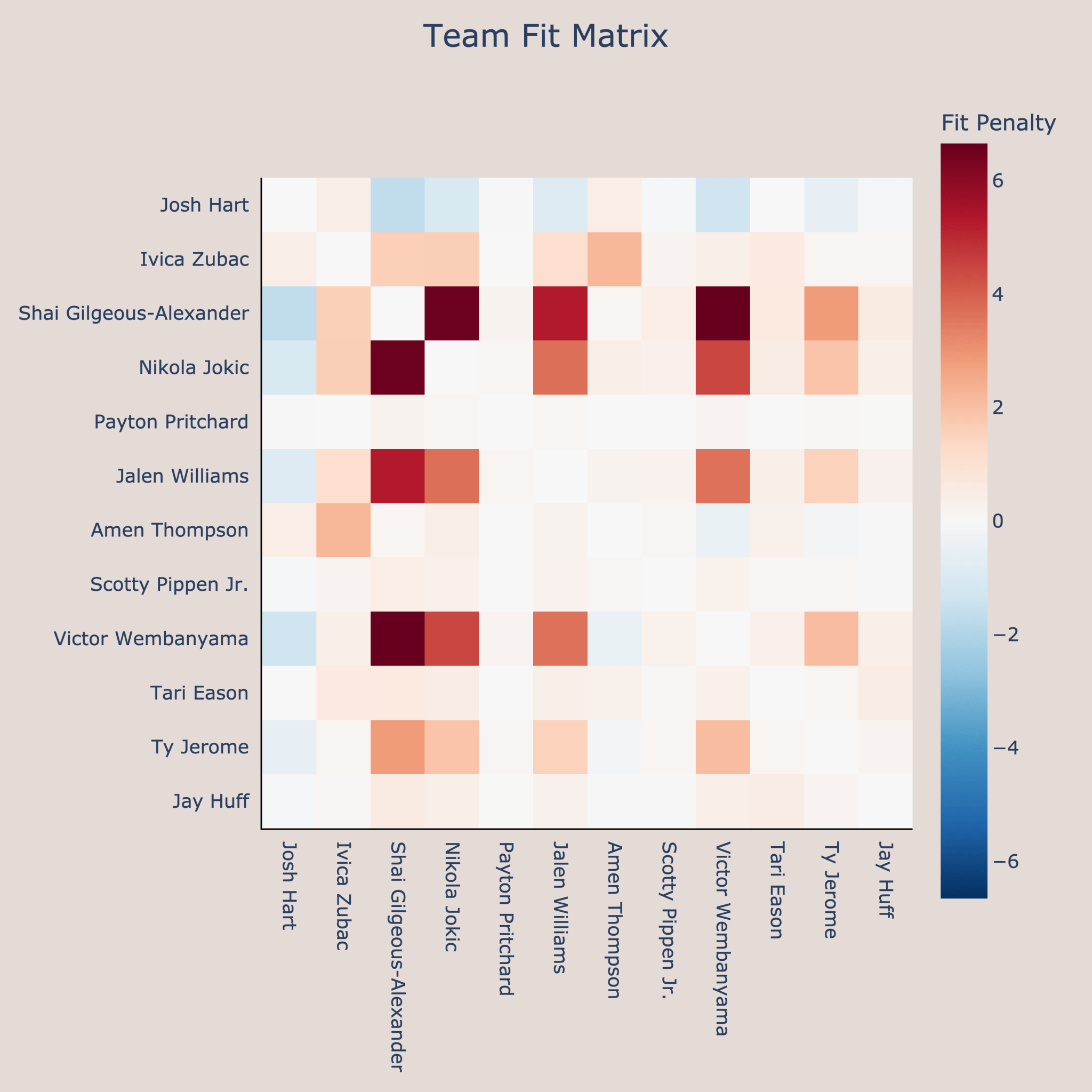
This roster is projected to win about 75 games4 while costing $187.5M, which is just under the luxury tax. It blends high usage shot creation stars with low usage specialists. Passing and defense are covered by players like Wembanyama, Eason, Pippen Jr., and Jerome. The shooting isn’t elite, but spacing is solid for everyone except Thompson and Hart. The stars drive the projected WAR, while the role players keep the fit penalty low by filling gaps in shooting, passing, and defense.
The fit matrix confirms that most penalties come from high-usage players, with role players rarely clashing.
Additionally, we see that the optimal team makes extensive use of rookie contracts to get effective players on small salaries. In the next section, we see how the optimal team would look if we don’t consider low cost rookie players.
Optimal NBA Team – No Rookie Contracts
Next, we remove rookie contracts from the player pool and build a roster using only veterans. This makes team construction tougher, since we lose the ability to get high-value players at low cost. Using the same roster size and salary constraints, but excluding rookies from the player pool, the algorithm produces the following team:

This lineup is projected to win 71 games while still costing about $187.5M. It leans heavily toward guards and bigs, with few true wings. That could reflect quirks in Basketball Reference’s WAR metric (possibly undervaluing wings), the fit penalty design (perhaps guards and bigs mesh better), or dynamics of the wing market (wings being overpaid relative to production). Whatever the cause, the overall pattern is familiar: a couple of high-usage stars surrounded by role players who bring passing, defense, and shooting.
Optimizing Free Agency Search
While building a perfect team from the entire NBA is fun, it’s not realistic as teams can’t just pick any player they want. A more practical use of the genetic algorithm is for free agency, where a front office needs to fill roster spots around a set core.
We can use the 2025 Philadelphia 76ers as an example. After losing many rotation players to free agency, suppose we keep only four core players5—Joel Embiid, Jared McCain, Tyrese Maxey, and Paul George—and try to fill the remaining spots exclusively with available free agents, staying under the luxury tax. The roster size limit remains 12, but the fitness function is modified so that any team missing one of the four core players gets a score of zero. The initial population is also generated with these players locked in.
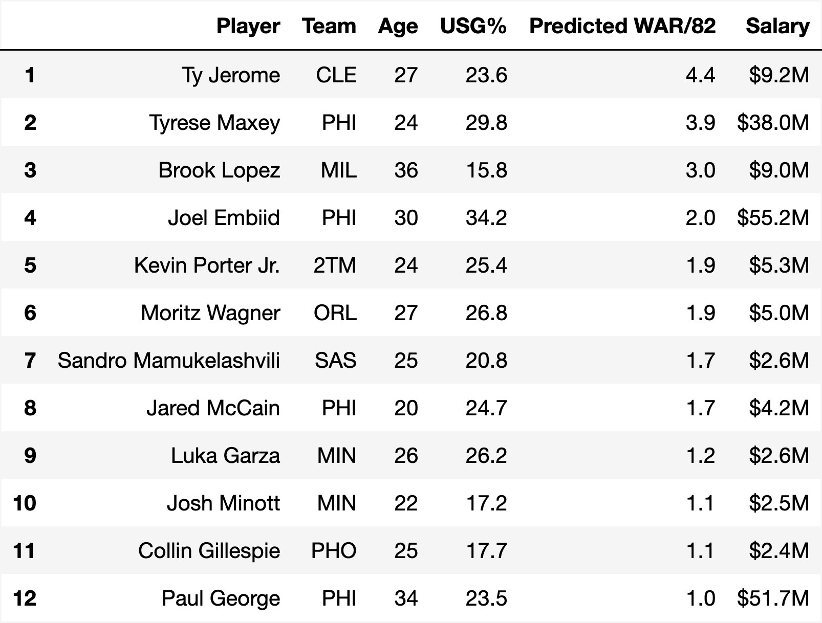
This lineup is projected to win 38 games, up from the team’s 24 wins last year. That’s likely an underestimate, since the WAR/82 model only uses one year of past data, and both Embiid and George are likely to bounce back from subpar seasons. Still, the constraints of keeping high salary stars and only signing free agents shape the roster heavily. With Maxey and Embiid as high-usage anchors, the algorithm surrounds them mostly with low-usage role players: Mamukelashvili, Gillespie, and Lopez for shooting; Porter and Jerome for passing; Wagner and Minott for defense.
Best Expansion Team
The final application is building an optimal expansion team, again optimizing only for the upcoming season. The key difference here is the available player pool. In an expansion draft, each existing team can protect a set number of players from selection. For simplicity, we allow each team to protect its top six players by projected WAR/82 for the following season. Rosters are taken as they stood before the offseason (e.g., Durant is still on the Suns).
This automated protection method produces an unrealistic but interesting list of available players, including Lu Dort, Alex Caruso, Chet Holmgren, Nickeil Alexander-Walker, Bradley Beal, Jerami Grant, and Jordan Clarkson. Because the process uses a single catch-all metric and ignores multi-year value, it can yield results that differ from realistic protection strategies.
Using this player pool, we construct a 12-man roster under the luxury tax:

This roster costs $145.4M and projects to win 35 games. It heavily draws from deep teams like the Thunder, Celtics, and Timberwolves, taking multiple players from each. In a real expansion draft, limits on players per team would prevent this; these rules could be added to the genetic algorithm, but require additional bookkeeping.
The roster notably lacks high-usage shot creators. Few quality options were available, and players like Beal or Clarkson were bypassed due to high salaries and low projected WAR. This underscores the challenge of building a playoff-caliber expansion team immediately. In practice, prioritizing youth and draft capital is a far more sustainable strategy.
Optimization is essential for achieving top performance with limited resources, and NBA teams are no exception. With a salary cap, they must assemble the strongest roster possible. Among the many optimization methods, genetic algorithms stand out for their flexibility, including the ability to factor in team fit penalties. Across the simulations, a common pattern emerges: a few star players surrounded by complementary role players who offer shooting, defense, and passing without demanding excessive usage. Building the perfect NBA team may be impossible, but genetic algorithms can bring us very close.
Footnotes
- This is similar to the knapsack problem but made more complex by considering player fit, which makes straightforward dynamic programming impractical ↩︎
- For the applications in this post, the penalty weight is set to 5. This means the fit penalty is multiplied by 5 before subtracting from the team’s total projected WAR/82 ↩︎
- The exact method for mapping fitness values to selection probabilities varies by problem. In my algorithm, I use a softmax function with a temperature parameter that decreases over generations ↩︎
- Calculation of 75 expected wins: The total predicted WAR/82 is 79.9. Dividing by 2.7 converts this to VORP per 82 games, yielding 29.6 points per 100 possessions better than a replacement-level team. Subtracting 10 accounts for the difference to an average team (since a replacement player is roughly 2 points per 100 worse than average, and there are always five players on the floor), resulting in 19.6 points better than average. Applying the Pythagorean wins formula then gives an estimate of 75 wins ↩︎
- This project excludes rookies, so V.J. Edgecombe is not included ↩︎
See the code to run the algorithms here: https://github.com/AyushBatra01/Genetic-Algorithms/tree/main
