
Being named an All-American is one of the highest honors for a college basketball player. The players that are named All-Americans are considered to be the best 15 players by 4 major groups. These include the Associated Press, United States Basketball Writers Association, Sporting News, and the National Association of Basketball Coaches. Each of these groups independently chooses their top 15 players of the season and places them into the first-team, second-team, or third-team. The ten players with the most votes (where votes are weighted with 3 points for first-team, 2 points for second-team, and 1 point for third-team) are given Consensus All-American honors.
In this project, I will use a neural network and a logistic regression to try to predict college basketball All-Americans based on their per-possession individual and team statistics. By training models using the last 12 years of college basketball data, we can get a good understanding of what statistics are indicative of All-American level players and use this information to predict which players will be All-Americans in the 2022-23 season.
Note: All stats and data are accurate through the morning of February 12, 2023.

Exploratory Analysis
Sample and Minutes
I chose to denote any player that received at least 1 vote from one of the four voting groups as an All-American. Having more All-American players allows for more positive results in the sample, since the fraction of college basketball players that get even 1 All-American vote is extremely low. This is helpful because it is already difficult to make good models when the number of positive results is so low.
I also needed to choose a minutes restriction. Since teams often play a different number of games, I measured minutes using Minutes Percentage. This statistic is used on various advanced college basketball statistics websites like KenPom and barttorvik. Minutes percentage represents the percentage of team minutes played and helps to even the playing field for players on teams with fewer games played. A histogram is good for showing the distribution of minutes percentage among All-American players.
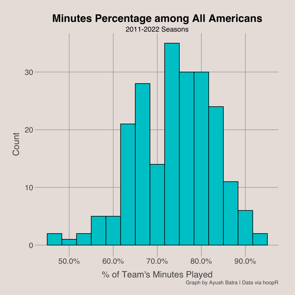
From the hisotgram above, we can see that most All-Americans played between 65% and 85% of their teams’ minutes. However, all All-Americans played at least 40% of available minutes. Therefore, I set the cut-off for minutes percentage at 40%.
Scoring

Scoring is the most important quality in the game of basketball. All good teams need players that can create shots for themselves and score when necessary. Therefore, it is obvious that players who are considered among the best in the country are very good scorers. This belief is confirmed by looking at the data.
The boxplot shows that the middle 50% of All-American scoring lies between 30 and about 36 points per 100 possessions, much greater than about 17 and 25, respectively, for non All-Americans. In fact, all but one All-American player (Kendall Marshall in 2012) scored over 20 points per 100 possessions, which translates to about 10 points in 30 minutes of a game at average pace.
Rebounding
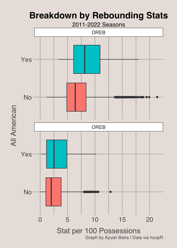
Rebounding is much less predictive of All-Americans than scoring. Although top players typically get slightly more offensive rebounds and defensive rebounds, the difference is not very big. In fact, there is a large overlap in the boxes representing the middle 50% of rebounding for All-Americans and non All-Americans.
Playmaking
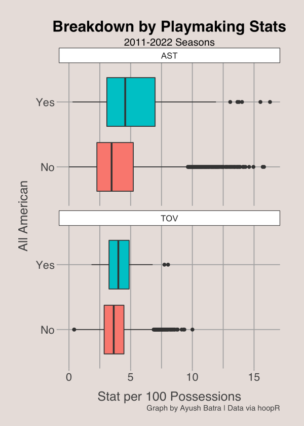
We can look at playmaking statistics like assists and turnovers as well. Neither statistic looks to be nearly as predictive as points, but All-Americans still have a greater median assists per 100. Even though turnovers are seen as a bad thing, All-Americans usually have more of them than those who didn’t receive a vote. The reason is likely that really good players usually have much higher usage rates, meaning they have the ball in their hands more often, giving them more chances to turn the ball over.
Defense

All-American players typically perform better than average on the defensive side of the ball. Blocks seem to be more predictive than steals are, meaning that the public likely values rim protectors over perimeter players that can disrupt passing lanes. Still, though, this plot shows us that voters do not value defense even close to how they value scoring when voting for All-Americans.
Shooting Efficiency
One would expect that All-American players shoot more efficient than others. The bar graph below shows the results. To ensure players who took few shots were excluded, I ensured that the included players must have over 50 attempts when counted for field goal attempts, 3-point attempts, or free throw attempts.
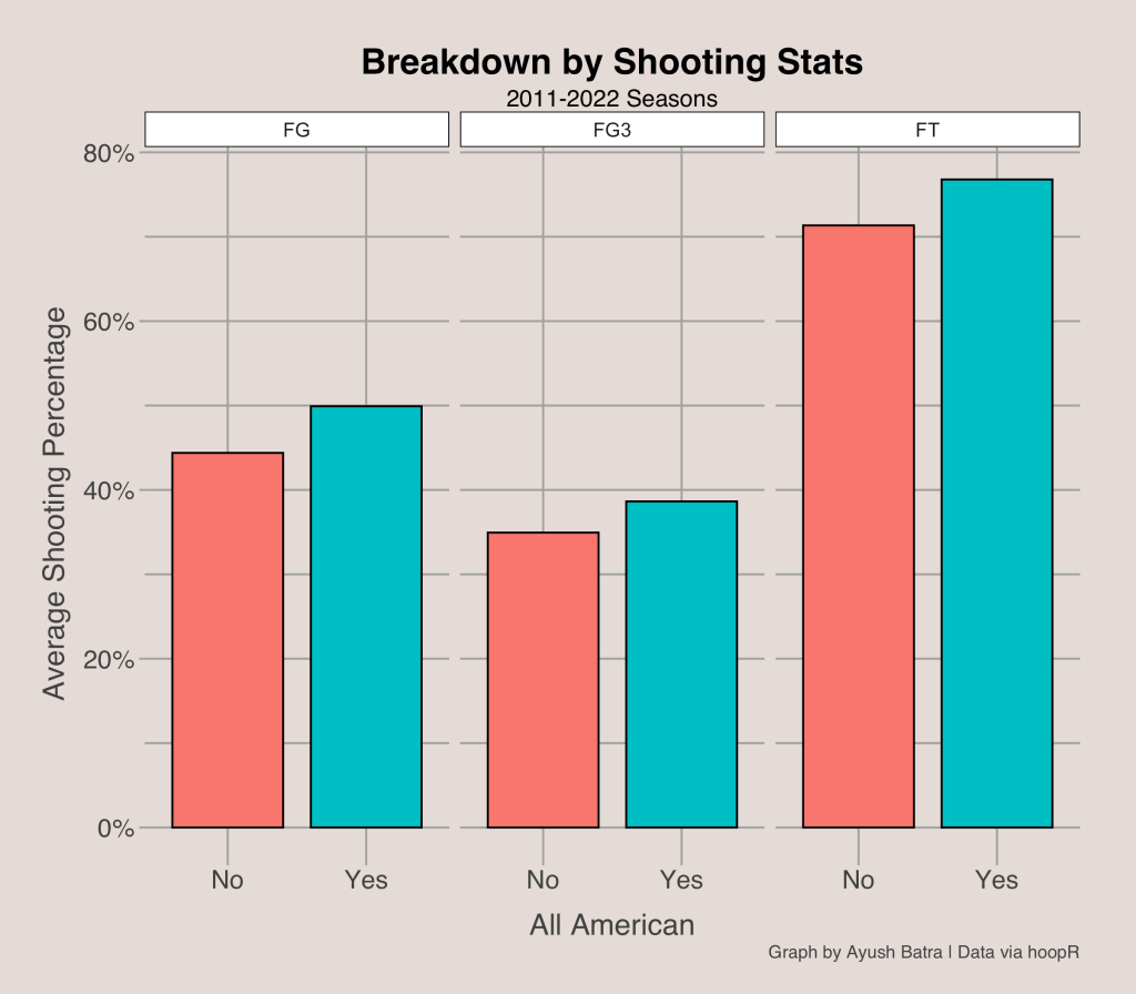
Indeed, All-Americans do shoot better than other players. The average field goal percentage for All-American players was close to 50%, while others were closer to 45%. In addition, All-American players that shot at least 50 3-point attempts had an average 3P% close to 39%. Free throws were also important as they shot an average of over 75% from the line. In comparison, players that did not receive an All-American vote shot about 35% and 71% on average on 3-point attempts and free throw attempts, respectively.
Team Efficiency Metrics
Next, we can look at team efficiency metrics and strength of schedule:

Team strength seems to have a large effect on the selection of All-American players. Almost all All-Americans are on teams that are among the top in the country, especially on offense. In fact, every single player that received at least 1 All-American vote since 2011 has been on an team with an adjusted offensive efficiency above the median. Defense is also important, but there were still some All-American players from below average defensive teams. Strength of schedule plays a role too, as All-American players played a tougher schedule than average. For those that watch college basketball, this is obvious as almost all All-American players come from teams that are top-8 seeds in the NCAA Tournament (implying they are among the top 32 of about 360 teams in the country).
The two most important variables in predicting All-Americans seem to be points and team quality. Let’s see how we can combine these variables to get an idea of what a typical All-American’s profile is.

The scatterplot above implies that most All-Americans are very good scorers and are on a very good team. It seems like a player needs to score at least 30 points per 100 or be on a team with an adjusted efficiency margin (adjusted offense – adjusted defense) above 20 to even have a chance of being an All-American. Furthermore, it seems that almost all high scorers on the very best teams are voted as All-Americans.
Additionally, the plot shows that we can predict All-Americans fairly well using just 2 variables. This could mean a couple things. One possibility is that the best players in college basketball are those that score the most points and play on the best teams. Another possible conclusion is that voters simply value scoring and team quality much more than anything else. The reality is likely a blend of the two as those who vote for All-Americans may not notice some more subtle qualities that more trained individuals like coaches do notice when measuring player performance. Awards voting in all sports has a skew towards winning teams, so its likely that voters overlook some incredibly deserving players on worse teams only because their team’s record is not very good or because they did not qualify for the NCAA Tournament.
Models
Neural Network
To get probablistic predictions for which players should be All-Americans, we can train a neural network. A neural network is a simple machine learning algorithm that “uses interconnected nodes or neurons in a layered structure that resembles the human brain.” A neural network is able to learn patterns in data by slowly improving accuracy over a series of many steps. The layers in neural networks make them suitable for complex modeling in relationships that are difficult to capture otherwise. Although predicting All-Americans is not complex enough that it absolutely needs to be modeled by a neural network, I thought it would be cool to try training a neural network with this data.
To train the network, I first separated the data into a training set, validation set, and test set. The training set is used to get the optimal weights in the model, the validation set is helpful in determining the best values for hyperparameters (like number of layers and nodes), and the test set is utilized to investigate how the model would perform on unseen data. In this exercise, I split the data into 70% for the training set and 15% for both the validation and test sets. Here is a quick summary of the positive results in each split (positive result = All-American):

After splitting the data, I scaled all the stats so they can be compared more easily. I did this using z-scores. A z-score can be calculated for a statistic by first subtracting the mean, then dividing by the standard deviation. This way, all statistics are in units of standard deviations and can be easily compared. For example, a z-score of 1 can be interpreted as 1 standard deviation above the mean. I trained the neural network with the scaled data. The network’s inputs included 2-point field goals made and attempted, 3-point field goals made and attempted, free throws made and attempted, offensive and defensive rebounds, assists, turnovers, steals, blocks (all in the form of per 100 possessions), team win percentage, adjusted offensive and defensive efficiency, and offense and defensive strength of schedule. The network had an input layer of length 17 and one hidden layer with five nodes.
After training the model and adjusting the hyperparameters, I applied the predictions to the test set. Some of these predictions can be seen below.

The root mean squared error (RMSE) on the test set was 0.0595, which is important to remember when comparing with the results of the logistic regression. A lower RMSE indicates better predictions. This RMSE value was actually lower than that for the validation set, conveying that the neural network can model the relationship between these statistics and the All-American status pretty well.
To get a better idea of the model’s performance, I looked at some false positive and false negative results. False negative results included players that actually got at least one All-American vote but had a low probability from the model. False positive results include players with a >50% probability of being an All-American according to the model but in reality did not get any votes.

Looking at the false negatives, we can get a sense of what the model sees as important. 3 of the 5 players with the lowest probabilities that actually got All-American votes were on mid-major teams, meaning they played inferior schedules to most All-American players. This means the model likely gives a high weight to team performance and strength of schedule. The 2 high-major false negatives were only voted as All-Americans by 1 of the 4 voting sites, so they were not seen as obvious All-Americans.
It seems that there were few extreme false positives in the test set as the highest probability for a false positive was just 76% while most were around 50%. This tells us that the model has a high specificity.
Now, we can apply the model to get predictions for this season. Using player and team stats up until the morning of February 12, 2023 can show us which players will likely make All-American teams.

Logistic Regression
We can also train a logistic regression using the same data. A logistic regression differs from a neural network in that it predicts a binary outcome similar to the way a multiple linear regression predicts a continuous variable. I wanted to train both a neural network and a logistic regression then compare results and see which model performed better.
Here are some of the training set predictions after training the logistic regression. The column “phat_nn” represents the predictions from the Neural Network while the “phat_logis” column represents predictions from the logistic regression.
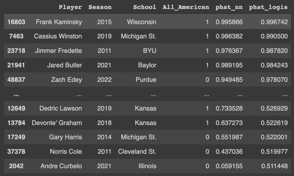
Looking at the results for the training set and test set tells us that the two models give similar probabilities for most players, but can vary a lot for others. For example, we can see above that Andre Curbelo in 2021 had an All-American chance of 6% according to the neural network and 51% from the logistic regression. I think most avid college basketball fans would agree that Curbelo wasn’t really a strong consideration for an All-American spot, so the neural network looks to be winning for this observation.
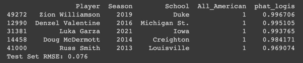
As shown below, we can see that the logistic model test set root mean squared error (RMSE) of 0.076 is greater than the test set RMSE of 0.0595 for the neural network. A lower RMSE indicates a better model, so it seems like the neural network made better predictions than the logistic regression.
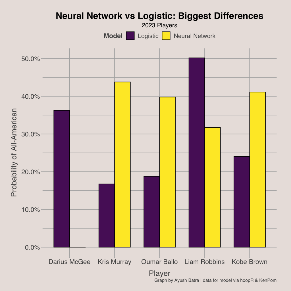
We can also apply the logistic regression model to this year’s players. Many of the results are similar, like how Edey, Tubelis, and Wilson are ahead of everyone else. However, there are a couple interesting results. Liam Robbins and Darius McGee both have high probabilities despite the fact that they likely will not be named All-Americans at the end of the season. Both play for teams that are not in the NCAA Tournament at-large picture, telling us that the logistic regression model probably does not give as much importance to team performance as the neural network does.

McGee and Robbins are two of the players with the greatest discrepancies in probability from the two models. They are joined by Kris Murray, Oumar Ballo, and Kobe Brown as the five players with the greatest difference in predictions from the neural network and logistic regression.
One advantage of a logistic regression is that it is easier to see which variables are the most important in determining the probability. The bar graph shows which variables have the greatest impact in the regression. We can do this because all of the independent variables are in a standardized scale, so the coefficients can be compared. In this context, the coefficient can be interpreted as how much the log odds would increase (or decrease) with a one standard deviation increase in the statistic. Note that the colors distinguish between the coefficients having a positive or negative sign. A positive coefficient means that having a higher value is better while a negative coefficient means having a lower value is better.

The graph reinforces some of the findings earlier, in that scoring and team performance are the most important factors in predicting All-Americans as 2-point makes, 3-point makes, win percentage, and free throws made are the 4 variables with the greatest coefficients. In additions, we can see that playmaking matters as assists is next.
There were some things that surprised me, though. First, both 2-point field goals made and 3-point field goals made had the same coefficient even though 3’s are worth more. This could indicate that 2-point scoring has increased importance in college. Additionally, shooting efficiency did not seem to matter very much as attempts in all shooting categories had very low coefficients (although this could be due to collinearity). We can see that the turnovers variable has a negative coefficient, so the model will give worse predictions to players with more turnovers, all other variables held constant. This is somewhat surprising considering All-Americans have a greater median turnovers per 100 than non All-Americans, but it’s what we want since turnovers are not good. Lastly, it seems that team offense is more important than team defense in this context since adjusted offensive efficiency and strength of opponent defense were more important than adjusted defensive efficiency and strength of opponent offense.

Improvements
My main purpose for this project was to compare the results of a neural network and logistic regression in a sports context. For this reason, I did not spend a lot of time on playing with which input variables led to the best results. Instead, I just chose to use all traditional box score stats scaled to 100 possessions for both models. I think the logistic regression fit could have been improved by using different combinations of variables instead of just using traditional box score statistics. For example, there could have been different findings if I used true shooting percentage or turnover rate or other more advanced metrics while dropping some of the simpler ones. However, the article was long enough, and I did not want to add a whole additional section about my variable choices in each model.
Conclusion
After investigating both the neural network and logistic regression, it seems like the neural network came up with the best predictions. Finally, we can see the projected All-American teams. If the season ended today, the first-team All-Americans would likely consist of Edey, Wilson, Tubelis, Jackson-Davis, and Miller. Unfortunately, this doesn’t account for positions as it is unlikely all 5 of these players will make the real first-team since all are forwards or centers. Marcus Sasser, Keyonte George, and Markquis Nowell headline the guards with highest All-American probabilities. The player with the greatest probability by a wide margin is Zach Edey, which is good since he is the NCAA player of the year favorite right now. In addition, all of the teams listed below except for Ohio State (Brice Sensabaugh) are on track to make the NCAA Tournament, reinforcing the belief that All-Americans play on high quality teams.


Watch out for these guys in the tournament come March!
See all the code and data here: https://github.com/AyushBatra15/All-Americans
Other Posts:
- Optimal NBA Team with Genetic Algorithms
- Mapping NBA Futures: Simulating Career Trajectories with WAR Projections
- Predicting Future Performance: The Best Shot Creators, Shooters, and Defenders in the 2024 NBA Draft
- Projecting Future All-Stars in the 2024 NBA Draft
- 2024 March Madness Predictions: Which Teams are Over and Under-seeded
