
The NBA Draft is approaching, and teams will be scouting players for specific skills that fit their needs. Some critical skills in basketball include creating shots, spacing the floor, and holding up defensively. While traditional scouting methods are important in identifying talent, they are somewhat inefficient as it’s not really possible to watch every second of every game for every prospect and maintain an unbiased thought process throughout. Statistical models can guide where to scout by pointing out players who are likely to succeed in any given area. In this project, I fit models to predict NBA outcomes that measure shot creation, shooting, and defense to find which what skills each player in the draft are expected to thrive at based on draft history.
Overview
As a quick summary, in this project I essentially fit models to predict six different NBA statistics: points per 36 minutes, true shooting percentage, assists per 36, turnover rate, 3-pointers made per 36, and defensive box plus minus. The first four stats help to measure creation, by taking into account both scoring and passing in addition to efficiency in both these areas. I measure shooting ability using 3-pointers made per 36 minutes, and I used this instead of 3-point percentage because I believe that shooting volume plays a major part in what makes a shooter dangerous. Lastly, I used defensive box plus minus as a measure for defensive ability because it is the best easily accessible all in one defensive metric. It is imperfect as it only relies on box score data when better estimates of defensive ability can be acquired using tracking data or on-off stats, but it was the best metric available for defense on Basketball Reference.
Data
Similar to my previous project on the NBA Draft, I used college data from prospects between the 2004 and 2020 NBA Drafts to fit the models. This data was webscraped from Tankathon.com. The stats for the 2024 prospects were webscraped from Tankathon as well. The NBA stats (which are used as response variables) were webscraped from Basketball Reference. Specifically, I scraped each player’s career NBA stats to get a wholistic view of their performance over time. Before apply any data transformations or fitting any models, I set a cutoff for 200 pre-draft minutes to be included in the analysis, so any players who played fewer than 200 minutes in their college / international / G-League season before the draft were not included due to lack of sufficient playing time.
Pre-Processing
Most of the pre-processing steps in this project were the same as in my previous draft project, so to get a more in-depth explanation of what I did, you can see there.
Feature Engineering
The initial dataset that I scraped from Tankathon included many traditional stats like points, assists, and rebounds, all normalized per 36 minutes. Additionally, it included advanced stats such as usage rate, true shooting percentage, and box plus minus while also providing biographical information like draft age, height, and wingspan. With this data, I created new features by transforming or combining the existing ones. For example, I created a variable for BMI using height and weight, and I also created variables to measure the difference between wingspan and height. I transformed traditional 3-point percentage into 3-point proficiency, which takes into account shooting volume in addition to shooting efficiency. I log transformed several variables with skewed distributions, such as assists and blocks, and other variables that make more sense on a log scale, like draft pick. Lastly, I created some interaction variables that I thought could be helpful for prediction for some of these models.
Train Test Split
I split the data into a training set and a testing set in order to be able to measure the generalizability of the models once they have been fit. I allocated 80% of the data to the training set and 20% to the testing set. There were 898 observations overall to begin with, and after splitting there were 718 samples in the training set and 180 in the testing set.
Imputation and Scaling
There was lots of missingness in the data that I scraped from Tankathon. Many non-college players did not have values for advanced stats like box plus minus or win shares, and several players were did not have a value for wingspan since I guess they were never measured. Therefore, I had to impute these values if I still wanted to use these variables but didn’t want to throw out data. To fill in these missing values, I used an iterative imputer. This works by estimating the missing values for one feature at a time using all the other ones and repeating for a set number of iterations. For this imputer, I capped the number of features used to 10 in order to avoid overfitting the imputed values.
After imputing missing values, I standardized all of the features, which means that they were linearly transformed so that the transformed means were 0 and the transformed standard deviations were 1. This allows each variable to be put on the same scale and is important to ensure equal weighing of features for regularization algorithms like LASSO or Ridge regression.
Modeling
Response Variable Shrinkage
All the response variables (points, true shooting percentage, assists, turnover rate, 3-pointers made, and defensive box plus minus) were continuous. One observation is that sometimes an NBA player will have an abnormally high value for one of these stats over their career because their career was very short. For example, a player may have played 5 total career NBA games and have a high career points per 36 because they happened to score a lot in their few NBA games. In these situations, the actual career statistic is not representative of the player’s skill, since they did not last in the NBA so they couldn’t have been that good. Therefore, I applied some form of shrinkage to all of the response variables so that players that played very little in the NBA had their career statistics shrunk towards some value. For counting stats (points, assists, and 3-pointers made), the stats were shrunk towards 0. For rate states (true shooting percentage, turnover rate, and defensive box plus minus), the values were shrunk towards some baseline. This baseline is meant to represent the average value of the stat for players that did not last in the NBA. I calculated this baseline by taking the average value of the stat for any players in the dataset that played fewer than 100 total career NBA games. For example, the baseline true shooting percentage was about 45%, since the average true shooting percentage for players drafted from 2004 to 2020 that played fewer than 100 career NBA games was about 45%. The baseline value for turnover rate was about 14%, and the baseline rate for defensive box plus minus was about -1.0. Again, the baseline for points, assists, and 3-pointers made per 36 were all 0 since those are counting stats.
The response variables were shrunk towards their baseline values using an exponential decay function. Here is the formula:

Here, “G” represents total career NBA games played and “adjusted” represents the response variable after shrinkage. This function allows the response variables for players with little NBA experience to be shrunk heavily towards the baseline, while players that played lots of NBA games will have very little shrinkage towards the baseline. Using this adjusted response value instead of the raw one will allows for better models since we are removing some of the noise that occurs in the NBA stats due to a low NBA career sample size.
LASSO Regression
The predictor variables included the standardized features scraped from Tankathon and created from feature engineering. Originally, I was going to fit a few different types of models for each response variable and choose the best one. However, when I tried this, the LASSO and Ridge regression models consistently had the best validation set scores across all the response variables. Both had similar performances, so I chose to go with a LASSO model for each response variable to keep consistency. Additionally, since LASSO regression penalizes the sum of the absolute values of the coefficients, it tends to shrink the coefficient values to zero, leading to a nice property where many of the coefficients are shrunk to zero and a few are not, which gives sparser and more interpretable models.
After deciding this, I fit a LASSO model for each response variable, each using the same pool of predictor variables. However, since there were a lot of predictor variables, even an L1 penalty led to a linear model with many non-zero coefficient values. In order to create simpler solutions, I fit another LASSO model, but this time using only the predictor variables whose coefficients were non-zero and large. To summarize, this is the process that I used to create the final LASSO model:
- First, fit a LASSO regression model for the response using all of the predictor variables; this will lead to a significant chunk of the coefficients being shrunk to 0
- After fitting the first LASSO model, I removed all of the predictors whose absolute coefficient value was less than 10% of the maximum absolute coefficient value. For example, if the largest absolute coefficient after the first LASSO model was 3, then I only kept predictor variables that had coefficients with an absolute value greater than 0.3
- Using this reduced set of features, I fit a second LASSO model, using the same response variable. This led to a few more features being shrunk to 0, allowing for an even sparser solution. This second model was the final LASSO model.
Interestingly, this method, which allows for slightly sparser solutions than the ordinary LASSO model, led to better validation results. In addition, it has the added benefit of being simpler since there are fewer features.
Results
The main focus of this project was to see which prospects are expected to excel in the NBA for some of the most important skills: scoring, passing, shooting, and defense. By training the models on several statistics and applying the results to the 2024 NBA draft class, we can find which players are expected to be the best at these skills.
Scoring
First, we can look at the results for the scoring model. I measured scoring using points per 36 minutes, so this model attempts to predict the future career points per 36 for the players in this year’s draft. To get some insights into the model, I have 4 visuals displayed below. The top left graph shows which features had the largest absolute coefficients. These are the traits that drive the predictions the most. On the top right, the training, validation, and test set losses are shown. Since this is a regression problem, the loss function I used was mean squared error. The main thing to look for here is how the test and validation loss compare to the training loss. If the test and validation losses are much larger than the training loss, then the model is generalizing poorly to unseen data and may be overfit. The bottom left and bottom right visuals display the players with the highest predicted points per 36 using this model for players in past drafts and players in this draft, respectively.

BPM: Box Plus Minus
PTS: Points (per 36)
log_MP: log transformed minutes played per game
na_bpm: dummy variable for if a player was missing box plus minus stats
There are many interesting results that can be seen from these model results. First, draft pick is the biggest driver of career points per 36, as players near the top of the draft are expected to score a lot more, which makes sense. Younger prospects that scored a lot (high PTS) and had a high impact (high BPM) were also expected to score a lot in the NBA. Looking towards this year’s draft, Reed Sheppard has the greatest expected points per 36 with a prediction of 17.9. For reference, Austin Reaves scored 17.8 points per 36 minutes last season. However, there is of course going to be some error with this prediction. For the test set, the standard deviation of the difference between the expected and actual points per 36 values was about 4.6, so there is a pretty large margin of error.
Photo Credit: Dylan Ballard – A Sea of Blue
Most of the expected top picks are the ones with the highest expected NBA career scoring numbers. An interesting exception is Matas Buzelis, who has an average draft board position of 5.6 but is not in the top 10 of expected points per 36 for this draft class. On the other hand, Jared McCain is in the top 10 for expected scoring despite having an average draft board position of 14.4.
Scoring Efficiency
Next we can look at scoring efficiency, as measured by true shooting percentage. True shooting percentage differs from traditional field goal percentage in that it takes into account both the value of 3-pointers and free throw shooting.

TS%: true shooting percentage
BPM: box plus minus
log_MP: log transformed minutes per game
eFG%: effective field goal percentage
C: dummy variable for the Center position
TO: turnovers (per 36)
na_bpm: dummy variable for if a player was missing box plus minus stats
3P%: 3-point proficiency
The best predictors of career NBA true shooting percentage were draft pick, draft age, 3-point percentage, and true shooting percentage. We expect highly drafted players that are young and had a good true shooting percentage before the NBA to be efficient scorers in the NBA as well. This model tends to penalize good perimeter shooters, as the predicted NBA true shooting percentage decreases as pre-NBA 3-point percentage increases. One result is that many of the players with the best predicted true shooting percentages are bigs who mostly play at the rim.
In this draft class, Donovan Clingan has the best predicted true shooting percentage (59.6%). We see lots of bigs at the top, like Clingan, Edey, and Missi, which is in line with the results from 2004 to 2023. The more intriguing results seem to be for the guards that appear in the top 10 for this year. We find that Reed Sheppard is expected to be an efficient scorer, which is logical given his efficiency at Kentucky. Zaccharie Risascher and Matas Buzelis are expected lottery picks with a low expected NBA efficiency. Risacher was missing BPM data and had a low imputed BPM, which along with a pretty high 3-point percentage (which is punished by this model) led to a low predicted true shooting percentage. Buzelis was not very efficient with the G-League Ignite and also had a low imputed Box Plus Minus, leading to a low expected NBA TS%.
Photo Credit: Jamie Squire/Getty Images
Passing

AST: Assists (per 36)
PG: dummy variable for Point Guard position
log_pick: log transformed draft pick
AST/USG: Assist percentage to usage rate ratio
AST/TO: Assist to turnover ratio
log_MP: log transformed minutes per game
Fouls: Personal Fouls (per 36)
AST_x_log_pick: interaction term between assists (per 36) and log transformed draft pick
To measure passing ability, I used assists per 36 minutes. The best predictors of NBA assists include draft pick, college assists, and position. We expect good passers in college to also be good passers in the NBA as most of the important coefficients have information about assists. Additionally, point guards get an extra boost compared to other positions, possibly because non-point guards have less of a creation burden in the NBA than they do in college. Three players are far above the rest in terms of expected assists per 36: Nikola Topic, Reed Sheppard, and Rob Dillingham. These players were very creative in college (or overseas, in Topic’s case) and should sustain that in the NBA. Possible lottery picks that are expected to be weak passers include Dalton Knecht, Alex Sarr, and Ja’Kobe Walter. These players should not be expected to be the main piece of an NBA offense; instead, they would be better utilized as off ball players due to their expected inability to create shots for teammates.
Photo Credit: FIBA Basketball
Turnovers
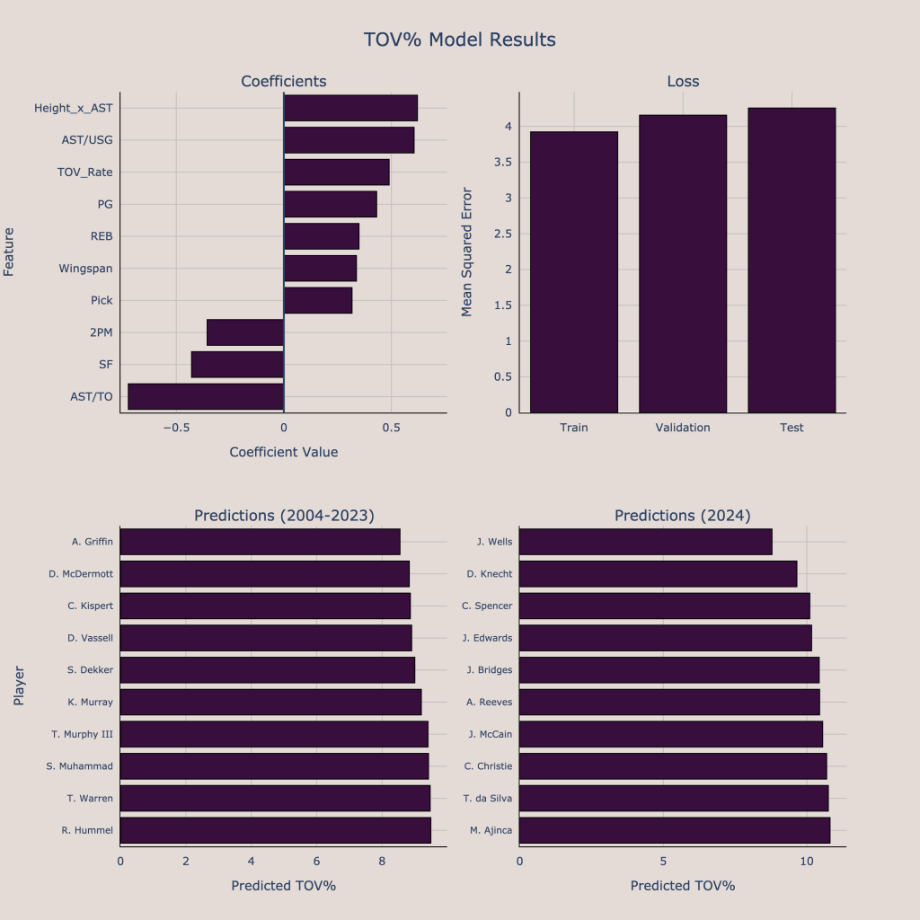
Height_x_AST: interaction term between height and assists (per 36)
AST/USG: Assist percentage to usage rate ratio
TOV_Rate: Turnover rate
PG: dummy variable for the Point Guard position
REB: Rebounds (per 36)
2PM: 2-pointers made (per 36)
SF: dummy variable for the Small Forward position
AST/TO: assist to turnover ratio
While passing and scoring is very important, it is also crucial to contribute to the offense while limiting turnovers. Therefore, we want to know how much players are expected to turn the ball over, as measured by turnover rate. The best predictors for NBA turnover rate are college passing and turnover stats. Players with a turnover issues in college (low AST/TO, high TOV Rate) and a perimeter-oriented game (low 2PM) are expected to be more turnover prone in the NBA. In this year’s draft, many of the players with a low expected turnover rate are players who should expect to have more off-ball roles in their NBA futures. Dalton Knecht and Jared McCain are two potential lottery picks who should have low turnover rates. Among potential lottery picks, Devin Carter, Nikola Topic, Reed Sheppard, and Rob Dillingham have the highest expected turnover rates. It is understandable that the players who are expected to be the best passers are also expected to have higher turnover rates since usually being a good passer means making riskier passes that could end up being stolen. However, Devin Carter’s high expected turnover rate is alarming since he doesn’t have nearly the projected passing upside that Topic, Sheppard, or Dillingham have.
Putting all of the four previous categories (scoring, scoring efficiency, passing, and turnovers) together, we can get a good idea of which players are most likely to contribute to shot creation. Reed Sheppard, Rob Dillingham, and Nikola Topic are expected to have a great passing numbers in addition to solid scoring numbers. Further down in the draft, Jared McCain presents an opportunity to grab a young player with scoring upside who is expected to be both an efficient scorer and a low turnover player. Players in the lottery who are not expected to be great shot creators include Risacher, Knecht, Buzelis, and Sarr as none of them were putting up big assist numbers before the draft, and being a good passer is often necessary to become the fulcrum of an offense in the NBA.
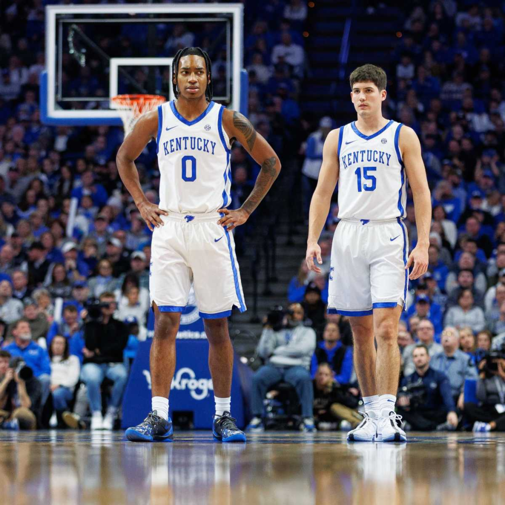
Photo Credit: Athlon Sports
Shooting

3PA: 3-pointers attempted (per 36)
FT%: free throw percentage
3PM: 3-pointers made (per 36)
BPM: Box Plus Minus
inv_pick: the inverse of the draft pick (1 / draft pick)
BLK_x_STL: interaction term between blocks (per 36) and steals (per 36)
Wingspan_diff: difference between Wingspan and Height
na_bpm: dummy variable for if a player is missing box plus minus data
An important swing skill in the NBA is shooting. If a player can’t shoot, then he has to be really good in almost every other area of the game to find time on the court. Therefore, being able to project shooting ability when drafting players is a must. The best predictors of 3-pointers made in the NBA are draft pick, 3-point attempts and makes in college, free throw percentage, and physical attributes. Players that shoot a lot and make a lot from the perimeter before the draft are usually dangerous shooters in the NBA. In addition, a high free throw percentage is an indicator of good shooting. Interestingly, height and wingspan are also important attributes as shorter players and more stocky players (low wingspan compared to their height) are expected to be better shooters.
In 2024, Jared McCain, Reed Sheppard, Rob Dillingham, and Dalton Knecht are expected to be the best shooters. All of them were high volume shooters in college and had good free throw percentages. Baylor Scheierman is a player who is expected to go in the late first round or early second round who also grades as a knockdown shooter. Johnny Furphy is another good shooter who is likely to be picked outside of the lottery. There are many players with alarming shooting numbers, however. Despite being labeled as a potential stretch big, Alex Sarr does not have a high projected three pointers made per 36. He had shaky shooting numbers (28% from 3, 71% at the free throw line) a made only 1.1 3’s per 36 minutes with Perth. Furthermore, his height and length are penalized by the model. Topić and Castle are guards that has shooting concerns, as neither was a very high volume or efficient perimeter shooter. The problem seems to be bigger for Castle, though, since Topić’s had a great free throw percentage (88%) and had a higher volume of 3-point shots than Castle did. Matas Buzelis has been labeled a potential shooter by some scouts, but his numbers also don’t look good as he only made 1.0 3’s per 36 and had less than a 70% free throw percentage with the G-League Ignite.

Photo Credit: Anabel Howery | The Chronicle
Defense

log_AST/USG: log transformed assist percentage to usage rate ratio
log_AST: log transformed assists per 36 minutes
PER: player efficiency rating
STL: steals (per 36)
PTS_x_log_pick: interaction term between points (per 36) and log transformed draft pick
log_MP: log transformed minutes per game
DBPM: defensive box plus minus
PTS: points (per 36)
AST/USG: Assist percentage to usage rate ratio
Lastly, we want to evaluate the defensive ability of players in the draft. It is important to not have any major defensive liabilities on a team, especially in the playoffs, so we need to evaluate how much of an impact each player has on defense. It is peculiar that assist numbers have high predictive ability in measuring future defensive box plus minus, since one would not think that passing and defense are very related to each other. Surprisingly, assist percentage to usage rate ratio is the variable with the largest impact in predicting this defensive metric.
Donovan Clingan projects as the best defender in 2024. Among lottery prospects, Reed Sheppard and Devin Carter project to be solid defenders at the guard position. This is somewhat surprising for Reed Sheppard, who has defensive questions due to his size, though he put up great defensive stats in college. After the lottery, Jonathan Mogbo, Ryan Dunn, and Adem Bona are players with defensive upside. Some lottery players with a poor defensive projections are Zaccharie Risacher, Dalton Knecht, and Rob Dillingham. None of them had great box score defensive metrics, so their projected defensive box plus minus stats are low.
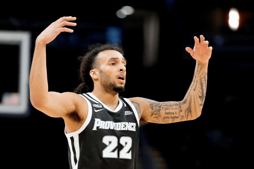
Photo Credit: Providence College Athletics
Summary
Now we have several models for different NBA stats that can tell us of a player’s creation, shooting, and defensive abilities. However, not all of the models will have the same amount of relative accuracy compared to just guessing the average value for each player. We can measure how much better each model is than random guessing by using the test score coefficient of determination. This number tells us the proportion of the variance in the dependent variable that is explained by the model, so a higher value means that the model is explaining more of the variation and is therefore performing better. The coefficients of determination are shown below.
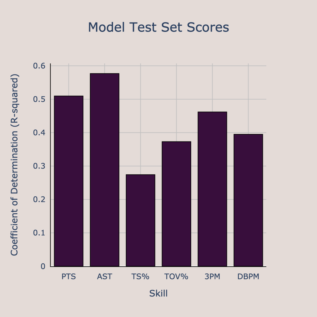
The models for assists, points, and 3-pointers made explain the most variance in their respective dependent variables, while the true shooting percentage model, turnover rate model, and defensive box plus minus model explain less variance. We are more confident in our predictions from the models for points, assists, and 3-pointers made since they are explaining more variance. In contrast, the models for the rate stats (TS%, TOV%, and DBPM) are not able to learn the data as well as these stats are more difficult to predict. This can have big implications on interpreting the model results. Since we should be less confident in the estimates for true shooting percentage and turnover rate but have higher confidence in the points and assists predictions, we should value players with high expected points and assists even if they may have a low expected true shooting percentage or turnover rate. Scoring and passing volume are much easier to predict than efficiency metrics, so subpar efficiency should not be enough to dissuade a team from taking a prospect alone.
After these analyses, we have a good idea of each player’s skills in the draft. The most high upside offensive players are Nikola Topic, Reed Sheppard, and Rob Dillingham due to their great passing stats and solid scoring projections. The most dangerous shooters are Jared McCain, Reed Sheppard, Rob Dillingham, and Dalton Knecht. On the defensive end, Donovan Clingan, Reed Sheppard, and Devin Carter project as positive defenders. Scouts are very good at picking out player strengths and weaknesses on their own, but using statistical models, we can get more precise and data-supported estimates for each prospect’s future NBA career.
See the code used for this analysis here: https://github.com/AyushBatra01/NBADraft
