Projecting Future All-Stars in the 2024 NBA Draft

The NBA Draft is an important time of the year for almost every team. Its a chance for teams to select their new face of the franchise and shape their future. Many of the high profile superstars were drafted to the teams they are on now. In fact, of the 15 players selected for an All-NBA team this past season, 7 (Jokic, Doncic, Tatum, Giannis, Edwards, Booker, Curry) are still on the team that drafted them, including 4 of the 5 first team All-NBA players. An even the ones that are not still on the team that drafted them had a large impact before they left their original team. The draft is critical for molding a team’s future image, so it is important to know what qualities lead to high-end NBA outcomes and which players are most likely to pan out as future All-Star level players.

In this project, I webscraped college stats and general player information for NBA players drafted between 2004 and 2023 from Tankathon.com, and I used this data to build a model that predicts which players have the best chance of becoming a future NBA All-Star and why.

Data

To acquire data that can be used to predict NBA outcomes, I webscraped information from Tankathon.com. This information included general player data such as height, weight, wingspan (if listed), draft age, and draft pick, along with the college/international statistics listed on the site. Specifically, I used the per 36 minutes stats instead of the per game stats in order to measure production per opportunity and not punish players that didn’t get as much playing time due to other circumstances. It also includes some advanced stats, such as usage rate, individual offensive and defensive rating, and box plus minus stats (although some of the advanced data is missing for international players). This data was collected for all drafted players between 2004 and 2023, inclusive, although only the data from 2004-2020 was used to train the model (since players after 2020 are too young and haven’t had many seasons to gain an All-Star appearance). I also webscraped the stats for players currently on the Tankathon.com big board for the 2024 NBA Draft. However, for the “draft pick” feature for 2024 prospects, I averaged the big board rankings from Tankathon, ESPN, CBS Sports, The Ringer, and Rookie Scale in order to create a more robust expected draft position (since obviously we don’t know each player’s draft pick yet). The response variable, or what we are trying to predict, is a binary response of whether or not the player has been named an All-Star at least once. This is imperfect as it is kind of a moving target since it is likely that some players that have been drafted between 2004 and 2020 may not have an All-Star appearance currently but will in the future, so this response is not a perfect indicator of a high-end NBA outcome but it is good enough and easily interpretable. I was able to find whether or not a player made at least one All-Star team by webscraping Basketball Reference.

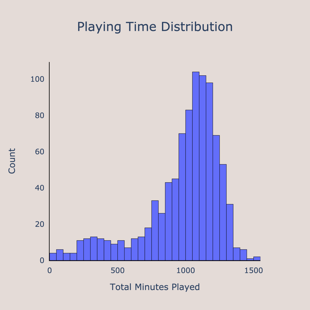
One main issue with the data was that some players had very little playing time in their year before the draft, meaning their production in limited time may not be indicative of their true performance. Therefore, I had to filter out players that did not cross some threshold of minutes played. After viewing the distribution of minutes played, I decided on a relatively relaxed cutoff of 200 minutes, meaning that any player had to play at least 200 minutes in their season before the draft (whether that be college, international, G league, or something else) in order to be included in the analysis. After filtering out players without enough playing time, there were 898 players left in the sample.

Pre-Processing

Feature Engineering

The initial dataset that was created by scraping Tankathon contained a lot of valuable information on counting stats and biographical information. However, by engineering additional features from the existing ones, it is possible to get even more information from this data when modeling. Some simple features that I created from existing ones included body mass index (BMI), Wingspan to Height ratio, and turnover rate (turnovers per 100 player “possessions”). Additionally, I transformed the listed positions into one-hot encodings. For players that had two positions listed, I assigned 0.5 to each position listed.

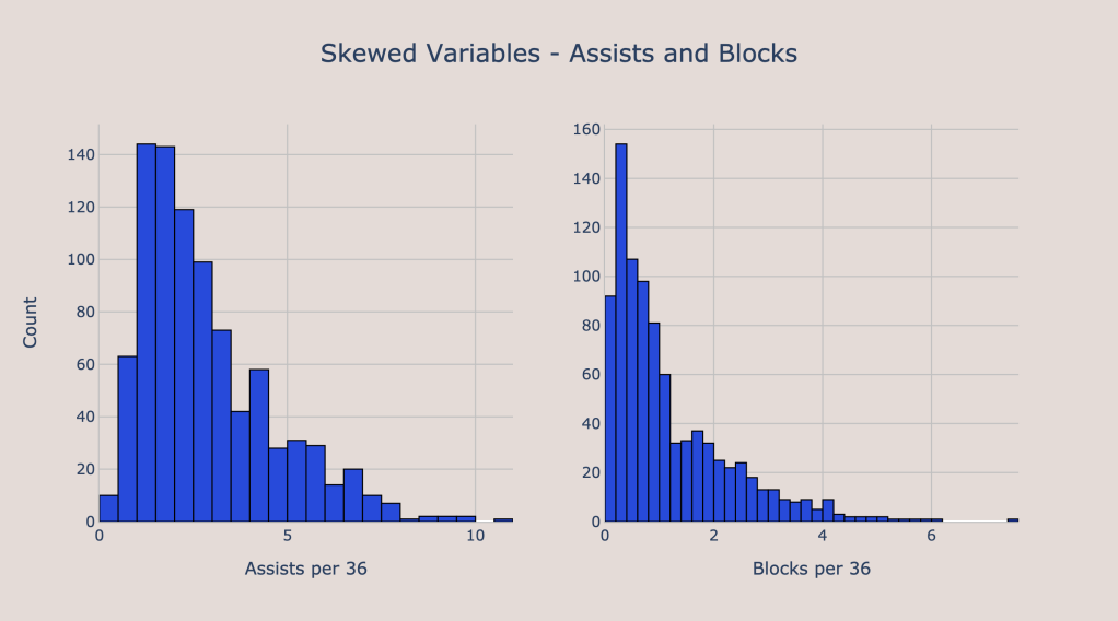
Many of the predictor variables that I used had very skewed distributions. For example, blocks and assists were two variables that had long right tails, as seen below. Therefore, I added predictors that corresponded to the log-transformations of these variables. Assists and blocks were not the only stats that were skewed — AST/USG (assist percentage to usage rate ratio) and AST/TO (assist to turnover ratio) were two other skewed variables. In addition, I also log transformed minutes played and draft pick. Minutes played was log transformed because I believe that each additional minute gives less information, and log transforming reflects that. I transformed draft pick because the difference between picks 1 and 6 is much larger than the difference between picks 31 and 36. Even though both are only 5 picks apart, the difference in talent level is much greater earlier in the draft, and the log transformation will ensure that this property holds while modeling outcomes.

Furthermore, another choice I made was to convert traditional 3-point percentage into a 3-point proficiency metric. Developed by Ben Taylor, 3-point proficiency accounts for both volume and efficiency from 3, so that players who take very few outside shots are punished. This helps to remove outliers that occur when a player has only taken a few shots and therefore has a heavily inflated 3-point percentage (an example is when a big has shot 1 3-pointer during the season and ends the season being 1 for 1, or 100%, from 3 despite taking only one shot). Lastly, I added some interaction terms that I thought would be relevant. Some of the interactions I added included an interaction between points and assists, height and assists, and 3-point proficiency and points.

Train Test Split

After the feature engineering steps, I split the predictor matrix and response vector into a training and test set. I used 80% of the data for training and 20% for the test set. After the split, the size of the training data was 718 observations, while the test set has 180 observations.

Imputation

A notable trait of this dataset is that there was a good bit of missing data. Many players, specifically the ones that did not play in college, were missing advanced stats such as box plus minus, win shares, and usage rate. Additionally, several players were missing data on their wingspans since I guess not all players were officially measured at the draft combine or some other event. In order to fill these missing values, I used an iterative imputer. This imputation method estimates the missing value of a feature using all other features by using one feature with missing values as the response at a time. For this imputer, I capped the number of features used to 10 in order to avoid overfitting the imputed values. The imputer was trained using the training data only.

Another important thing is that these data were not missing at random, since the players missing data primarily consisted of those who did not play in college. Therefore, I added an indicator variable for whether a player was missing some type of data to account for a potential bias. The fact that the data is not missing at random does mean that these imputed values may be biased, but I feel that it is better to include the data with some bias, since it can still have predictive value, rather than get rid of it all together.

Scaling and Dimensionality Reduction

I standardized all the variables so that each predictor had a mean of 0 and a standard deviation of 1 after imputation in order to put all the variables on the same scale. After scaling, I applied Principal Component Analysis to the dataset in order to reduce the dimensionality in a way that keeps the directions explaining the most variation in the data. Apply the PCA to the training dataset, one can see how much each additional component explains variation in the data, which can help to get an idea of how many features to keep. I decided to keep 15 features since that amount explained over 90% of the variability in the data while reducing the amount of features to a more manageable number.

Modeling

After imputation and scaling, I went to model training and tuning with the goal of predicting the probability of a player becoming an NBA All-Star. I trained six different models: a logistic regression with L1 regularization, a logistic regression with L2 regularization, a decision tree, a random forest, a naive bayes model, and an XGBoost classifier. For each of these models, I used a grid search with 10-fold cross validation on the training set to optimize the relevant hyperparameters. The optimized hyperparameters included regularization strength for the logistic regression models, the depth and splitting criteria for the decision tree, the number of trees and depths for the random forest, and regularization and subsampling parameters for the XGBoost classifier. All of these hyperparameters were tuned using cross validation to prevent overfitting the models.

To choose the final model, I examined the training and cross validation losses of each one. The loss function that I used was log loss, which measures how far the model predictions were from the actual observed results. Log loss is a commonly used loss function for classification problems and heavily penalizes predictions that are very incorrect (for example, if the model predicted a player would be an All-Star with probability 0.0001% but the player ended up being an All-Star, then the log loss of that single observation would be massive). A lower value for log loss indicates a better performing model. In addition, we want to avoid models with a large gap between training performance and validation performance because a much better training performance indicates that the model is likely overfit and will generalize poorly to unseen data.

Based on the cross validation losses and the degree of overfitting for each of the models, the best choice is either logistic regression with L1 regularization or logistic regression with L2 regularization. Their performance looks almost identical in the graph above, so we can look at the exact cross validation loss values to see which performed better.

Although the logistic regression with L2 regularization performed slightly better than the other logistic regression model in cross validation, the improvement in performance of switching from the L1 logistic regression to the L2 logistic regression is just 0.5%. Therefore, it seems that the difference in validation performance between the two logistic regression models is negligible. Since regression with an L1 penalty tends to lead to sparser, and therefore more interpretable, models, I chose to go with the logistic regression with L1 regularization as the final model.

Final Model

Instead of using a single L1 regularized logistic regression model, I chose to use bagging to create a more robust model that can give further insight into variable importance and prediction reliability. Bagging, which means bootstrapped aggregating, is an ensemble learning technique that involves repeatedly resampling the data with replacement (bootstrapping) and refitting the given model for each resampled data set, while making predictions by aggregating the results from every model. After fitting the bagged logistic regression, I evaluated the results on the training set, the cross validated set, and the test set.

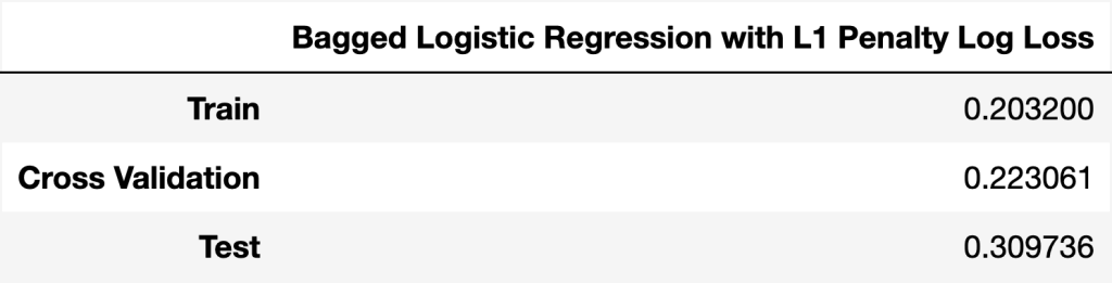
The validation and train errors are similar to what was seen previous for the logistic regression with L1 regularization, although both losses are a tiny bit lower. The test set loss, which I only evaluated after choosing and fitting the final model, is much higher than what would be expected from the validation loss. This could be due to an unlucky train test split, though another possibility is that the low validation set sample sizes in cross validation are leading to loss estimates with high variance and resulting in an optimized hyperparameter value that is not actually optimal.

For classification problems, it is crucial to have a well-calibrated model. A model that is well-calibrated ensures that the probabilities given to observations are consistent with what is observed. For example, a well-calibrated model that predicts a 70% chance of some outcome will actually see that outcome happen about 70% of the time. One way to assess model calibration is to put samples with similar predicted probabilities into buckets and see how the actual proportion of players that have at least one All-Star appearance compares to the average predicted probability of the observations in the bin. If the probabilities match up, then the model is well-calibrated. The figure below displays the actual results compared to the average predicted probability in each bucket, and the dotted line represents what we would see for a perfectly calibrated model. The blue line is very close to the dotted line, indicating that the bagged logistic regression model is well-calibrated and its predictions are consistent with what actually ends up happening.

Feature Importance

Using the bagged L1 regularized logistic regression model, we can find out which features have the biggest impact on the results. Since this model took in the PCA components as inputs instead of the original features themselves, we first must see which PCA components were the most important. In a regression model with a L1 regularization, it is likely that at least some of the features will be shrunk to 0, so one way to figure out feature importance is to see what proportion of the time each PCA component feature was shrunk to 0 in the bagged model (since the bagged regression consists of several models fit on bootstrapped samples).

Another way of measuring feature importance is to simply take the average coefficient values of the bagged regression models.

Examining the two above visuals, it seems like the two most important features were the 4th and 2nd PCA components. Each PCA component is a linear combination of the (scaled) features, so we can see which features tend to be driving the model. The 6 features with the most positive contributions and negative contributions to the 4th PCA component are shown below.

When this component is positive, it boosts a player’s predicted probability of being an All-Star. The component is driven by a low draft pick (low in the numerical sense, as in 1 is lower than 60), a low draft age, low shooting efficiency, (eFG%) high usage (USG%), shooting potential (3PA and the 3P%_x_PTS interaction), and physical traits (WS/Ht and Wingspan difference). This tells us that young highly ranked prospects with high usage, shooting potential, and a long wingspan are more likely to become All Stars. The players between 2004 and 2020 that had the highest values for this PCA component included Kevin Durant, Anthony Edwards, Andrew Wiggins, Jaylen Brown, and Brandon Ingram.

The 2nd most important PCA component is the 2nd PCA component. We can break down this component in the same way as before. As seen below, PCA component 2 is driven by having lots of turnovers (TOV) and assists (AST) along with few 3-point shots and attempts. Basically, this component will be greater for non-shooting playmakers. The players between 2004 and 2020 with the most positive values for this component included Ricky Rubio, Kendall Marshall, Ja Morant, Marcus Williams, and Michael Carter-Williams. It seems odd that this component is so important when many of the players that score highly in this component did not end up becoming All-Stars. For example, among the 20 players with the highest values for PCA component 2, only Ja Morant, John Wall, Ben Simmons, and Mike Conley became All-Stars.

Predictions

Now that the model has been fit and we can understand which features are driving the predictions, we can apply the model to get All-Star probabilities for draft prospects. First, to get an idea of what the model would have predicted in the past, we can look at the players between 2004 and 2023 with the greatest All-Star probabilities.

Among the list above, only Ricky Rubio and Markelle Fultz have played several years and did not end up being All-Stars. Victor Wembanyama has only completed his rookie year, but it would be surprising if he is not named an All-Star in the near future. From examining these predictions, the good news is that the model does a solid job at its task: to predict future All-Stars. However, one drawback is that a lot of NBA players that are named All-Stars don’t end up become franchise changing superstars that teams often hope for in the draft. For example, while John Wall and Ben Simmons were good players, neither ended up leading their team further than the second round of the playoffs. However, both were very impactful NBA players and gave the Wizards and 76ers, respectively, several years of high level basketball.

Now, finally, we can apply the predictive model to the draft prospects for the 2024 NBA Draft. First, we can get an overall idea of which players are most likely to be named All-Stars at least once by seeing the players with the greatest predicted probability. Using this model, Nikola Topic has the best chance of being an All-Star, although the model only gives him a 34% chance of it. This is pretty low compared to the players with the best chance of being All-Stars in past drafts. In fact, only the 2013, 2006, and 2004 drafts had a maximum predicted probability of being an All-Star lower than 50%, reinforcing the overall consensus that this year’s draft class is very weak, especially at the top. Still, Nikola Topic would be a high upside pick and possibly a bargain if his draft stock falls due to injury. The five players with the highest upside given by the model are Nikola Topic, Alex Sarr, Stephon Castle, Zaccharie Risacher, and Donovan Clingan.

A more robust way to investigate these predictions is to take advantage of the variety of models created using bagging. By getting the predictions from each model fitted on resampled data, we can get a range of predicted probabilities, which can help us get an idea of how confident these predictions are. Below, you can see the bagged predictions for the top 15 players in the 2024 NBA Draft, as measured by average draft board position.

There are lots of insights from this visual, but one of the most important ones is that the predictions for the players at the top have wide intervals, indicating a low degree of confidence in these predictions. This means that we don’t really know which player has the highest chance of being an All-Star for certain. Looking at the box plots, it seems like the five players mentioned previously are all pretty close to each other with their predictions. Another notable feature is that Reed Sheppard seems to have a low chance of being an All-Star. This is because of he has a low value for PCA component 4, which is usually greatest for players with long wingspan, high usage, and inefficient scoring. Sheppard had a relatively low usage rate (18%), does not have outstanding physical attributes (6’3″ tall with a 6’3.25″ wingspan), and was one of the most efficient players in college basketball (68% eFG%), so it makes sense that he has a low PCA component 4 value. As mentioned previously, the 4th PCA component has the largest impact in the model, so Reed Sheppard’s low value for this feature is driving his predicted All-Star probability down.

In the later portion of the lottery, it seems like Buzelis, Dilllingham, Holland, Salaun, Williams, and Walter all have similar chances of becoming All-Stars. The players with notably lower probabilities are Knecht, McCain, and Carter. While all of these players could become solid NBA players, these three have a lower ceiling due to either age (for Knecht and Carter) or low assist numbers (McCain and Knecht). Teams looking for high floor, low ceiling players that are more likely to be ready to contribute to a team immediately should target Jared McCain, Dalton Knecht, and Devin Carter, while other teams looking for more of a star player should pick someone else.

Takeaways

By fitting a model to predict future NBA All-Stars and applying it to previous years along with this year, we can gain insights into the process of predicting future NBA outcomes. First, it is difficult to project draft prospects. The large range of predictions suggests that there is high uncertainty in these predictions. While the players at the top of the draft tend to be better than players selected later, there is not much of a difference between players that are drafted in close ranges. By examining the PCA components that had the highest predictive value, we can get an idea of what traits correspond to high ceilings in the NBA. The 4th PCA component, which had the largest impact on predictions, was most heavily influenced by draft pick, shooting, usage, and physical traits. The 2nd PCA component, which was the next most important, was influenced by playmaking metrics like assists and turnovers in addition to shooting stats. Since the draft pick had a high impact, we can see that draft scouts do a good job of identifying talented players who have a solid chance of becoming future All-Stars. Additionally, the impact of physical traits, like wingspan to height ratio, inform us that it is more important to have a long wingspan than to be a tall player. Lastly, it seems that playmaking is more predictive of future high-end NBA success than scoring is, so it is better if a player shows playmaking promise with high assist numbers. Ideally, the best prospects are highly touted by scouts, have a long wingspan relative to their height, and show an ability to create shots for others.

See the code used for the analysis here: https://github.com/AyushBatra01/NBADraft