
The bracket for the 2024 NCAA Men’s Basketball Tournament has been released, and I have run 100,000 simulations of my college basketball ranking model to estimate the probabilities of each team advancing to each round. From this, some possible sleeper teams, upset picks, and title favorites can be examined.
Modified Elo Rating System: ELASTIC Ratings
My new college basketball ranking system is called ELASTIC: Elo adjusting for LocAtion, ShooTIng, and sCore (not a great acronym, but more catchy than just using “Elo”). As suggested by the acronym, this is an Elo rating system that is modified with a few extra features to better capture basketball performance.
Traditional Elo
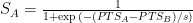
Here is how an Elo rating system works. To begin, we set each school’s team rating as 1500 (this number doesn’t mean anything, but is instead only meaningful in comparing schools; 1500 is used as a starting point by convention). To get the win probability for a team in a game, you first find the ratings for both teams (


From this equation, one can see that a greater difference in ratings between team A and team B will lead to a greater win probability for team A. Then, after seeing the result of the match, the ratings for both teams are updated. The updating formula is as follows:

where 
Modifications
Decaying K-factor
I made a few modifications to the traditional Elo rating system to get better results. The first modification I made was to have a variable K-factor. The K-factor is responsible for how much a team’s rating is updated based on the result of the game. At the beginning of each season, the K-factor is very high since teams change from year to year and we want to quickly capture how a team has changed from the previous season. The K-factor decays exponentially towards a set minimum as more and more games are played. Specifically, the K-factor for a team’s nth game of the season can be calculated as follows:

The Kmin, Kmax, and decay rate are hyper parameters that must be tuned. For this college basketball model, the Kmax is 206.5, the Kmin is 32.8, and the decay rate is 0.123. Using these numbers, the K-factor for each team will be as follows for each game of the season.

It is important to note that the game number resets at the beginning of each season.
Note: This decaying k factor is not an original idea (someone else originally thought of this and I am just applying it to the model since it works well)
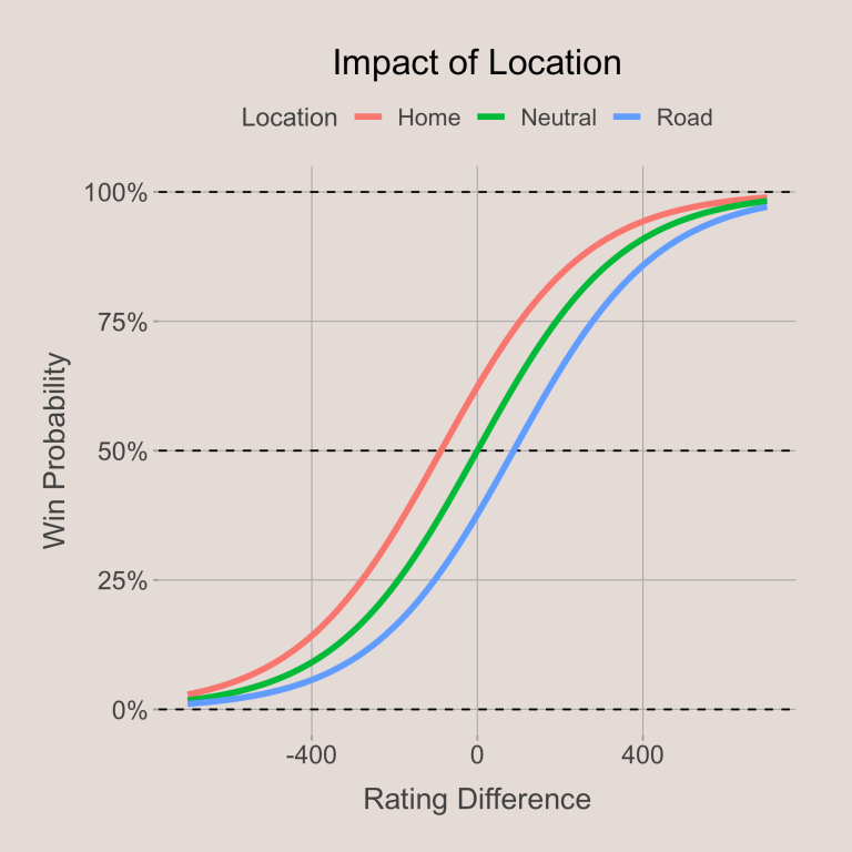
Adjusting for Location
Another important element to control for when predicting college basketball games is location. Teams are much more likely to win at home than they are to win on the road. To control for location, I added another hyper parameter: 

For the college basketball model, the home factor (
Adjusting for Score
Most analytical team ratings use some form of point differential (most often, they use points per 100 possessions) instead of simple win-loss results since beating a team by 30 is not the same as beating a team by 1. This, I believe, is the primary weakness of using a traditional Elo model to predict college basketball results. Therefore, I made some changes to incorporate information from the score.
In traditional Elo, the game score (SA or SB) for a team is either 1 or 0, depending on if the team won or lost, respectively. To incorporate the point differential of the game, I modified SA and SB so that they can take any values between 0 and 1, where the value depends on the point differential. When team A beats team B by a lot, the score for team A (SA) will be close to 1; when team A loses to team B by a lot, SA will be close to 0; and when the game between team A and team B is very tight and decided by just a few points, the both SA and SB will be near 0.5. I did this by applying the sigmoid function to a number proportional to the point differential of the game. Specifically, the score for team A will be as following:
I found that the best value for s, the scaling factor, was 5.2 (shown in graph below). This scaling factor controls the sigmoid curve’s shape. A greater scaling factor will make the sigmoid function more spread out and increase the importance of point differential, while the opposite is true for a lower scaling factor.
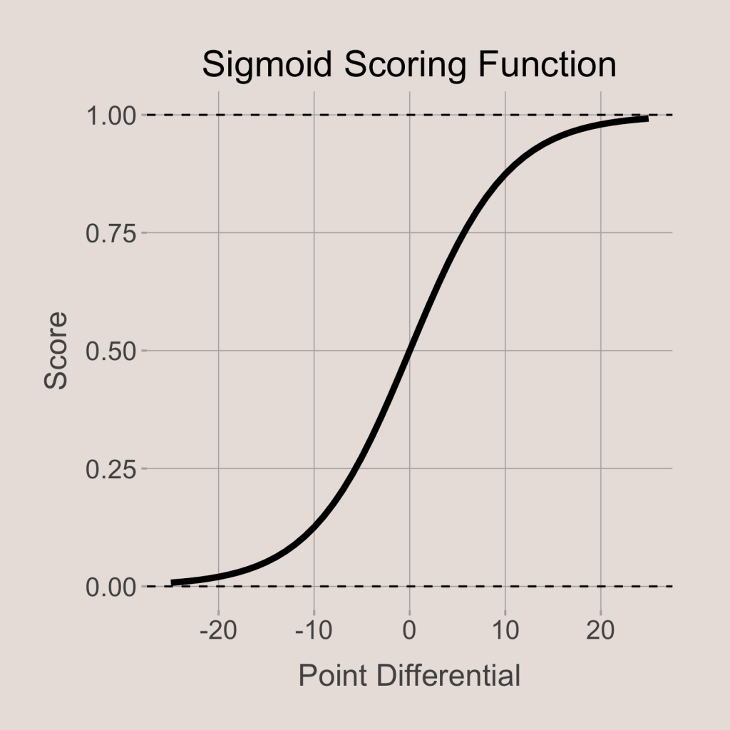
Using a sigmoid function to modify point differential has another bonus: winning by an additional point has a decreasing impact on the score. Basically, this means that winning by 10 is a lot better than winning by 5, but winning by 25 is basically the same as winning by 20. This helps account for the fact that once teams are winning by a lot, they aren’t really trying to continue to run up the score (instead they drain the clock, put bench players in, etc.). Including point differential into the Elo rating updates allows for us to reward teams for winning by a lot without giving too much credit for blowouts.
Adjusting for Shooting
The final adjustment I made was to account for a bit of shooting luck when looking at the point differential. This works by looking at a the opponent’s 3-point percentage and free throw percentage, shrinking those figures towards the NCAA average 3-point percentage and free throw percentage, then recalculating the opponent’s points based on the altered shooting percentages and using the result in the sigmoid scoring function. The amount to which the 3-point percentage and free throw percentage are shrunk towards their respective means are hyper parameters (one for 3-point% and one for free throw%). This is only done for the opponent’s shooting numbers because 3-point defense is very inconsistent and results are usually more due to luck than actual skill in defending the 3-point line.
To make sense of this, consider the following example: Team A scores 70 points and Team B scores 60 points. Let’s say that Team B shot 3/20 from the 3-point line and 15/30 from the 3-point line. A 15% 3-point percentage and 50% free throw percentage are terrible numbers, so Team A was pretty lucky in this game defensively. Let’s say that the 3-point shrinkage factor is 0.3, the free throw shrinkage factor is 0.75, the average NCAA 3-point percentage is 35% and the average NCAA free throw percentage is 70%. The adjusted 3P% for Team B will be shrunk towards the average, and using the numbers given above it will be [3P shrinkage factor * actual 3P% + (1 – 3P shrinkage factor) * average 3P%] = 0.3 * 35% + 0.7 * 15% = 21%. The adjusted FT% for Team B will be shrunk towards the average in the same way, so it will be 0.75 * 70% + 0.25 * 50% = 65%. Then, we can recalculate the points for Team B by doing the following: [actual points + 3 * (adjusted 3P% – actual 3P%) * (actual 3P attempts) + (adjusted FT% – actual FT%) * (actual FT attempts) ]. This comes out to be 60 + 3 * (0.21 – 0.15) * (20) + (0.65 – 0.5) * (30) = 60 + 3.6 + 4.5 = 68.1. So Team B’s adjusted number of points is 68.1. We consider this to be Team B’s score when evaluating Team A. That means that the point differential for Team A would be 70 – 68.1 = 1.9. However, Team B having 68.1 adjusted points is considered only from the perspective of evaluating Team A; from the perspective of evaluating Team B, these shooting numbers are taken as a sign of bad offense as opposed to unluckiness. Some extra steps are taken in the actual code I implemented to ensure the score for A and the score for B sum to 1, but this is the overall idea.
The 3-point shrinkage factor for this model ended up being 0.327 and the free throw shrinkage factor is 0.728. This means that free throw percentage is shrunk more to the mean than 3-point percentage is, implying that defenses are less in control of opponent free throw accuracy than opponents 3-point accuracy (this makes sense). In addition, we see that the 3-point shrinkage factor is not super high, suggesting that teams have a solid amount of control over opponent 3-point accuracy, though there is still lots of luck involved. You can see how the opponent’s points would be adjusted for possible 3-point and free throw percentages given the actual shrinkage factors of the model for a NCAA average number of 3-point and free throw attempts.

Future Improvements
Preseason Ratings
There are some improvements that I would like to make on the ELASTIC (Elo adjusting for location, shooting, and score) ratings. First, the ratings would likely be much better if I could include some kind of preseason prior. Currently, the prior for each season is the final rating from the season before. However, personnel changes and player movement mean that teams may be very different from one year to the next, and it may not make sense to expect them to perform the same way. In the future, I hope to use qualities like returning minutes and incoming roster talent to make preseason priors that hopefully perform better than just using the previous season’s rating.
Injury Adjustments
Often times, a team will suffer a big injury that impacts their performance in a big way. Betting markets and fans know that a team with a key player sidelined due to injury is not likely to be as good, but the ELASTIC ratings don’t know this since there is nothing marking an injured player. In the future, I would like to keep track of injured players in some way and modify the win probabilities based on injury information.
Per-Possession Numbers
Lastly, it may be a good idea for me to use per-possession numbers instead of point differential. Right now, I use point differential to determine the score of a game mostly because it is convenient. It would be interesting to see if using points per 100 possessions within a single game performs better than point differential or not.
Data
I got the data for game by game results using the hoopr package. The elo model was ran using all NCAA basketball games with at least 1 division I team since the 2010-11 season.
ELASTIC Rankings
Top 25
Now that the rating system has been explained, here are the current top 25 teams in ELASTIC.
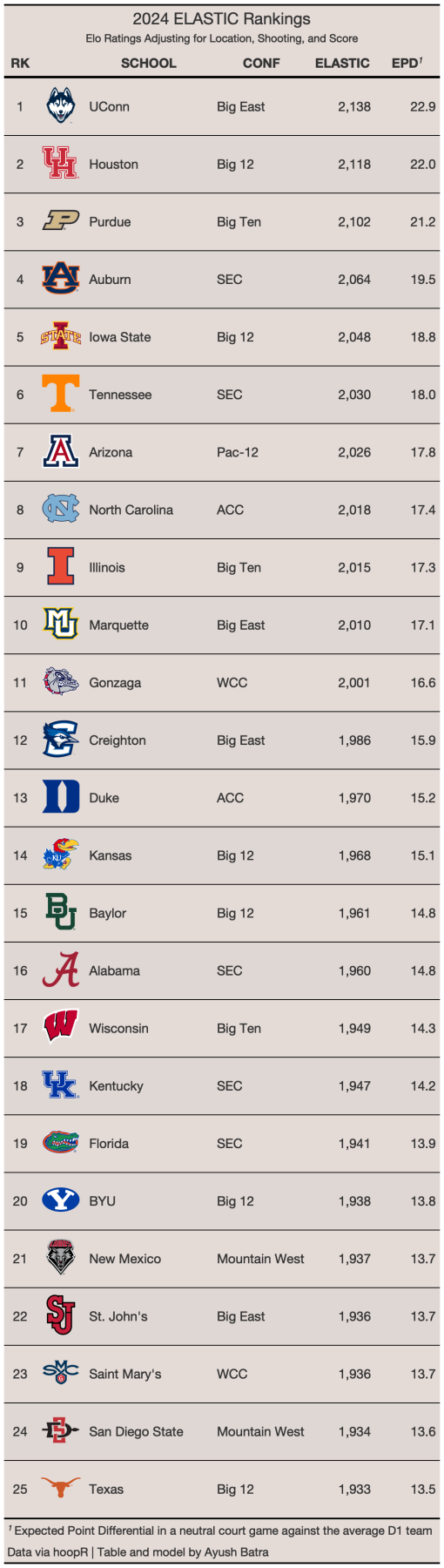
I included a column displaying the expected point differential (EPD) in a neutral court game against the average D1 team since I felt it may be a more meaningful number than the ELASTIC rating number itself. This top 25 looks similar to other ranking systems like KenPom, ESPN BPI, and barttorvik. UConn, Purdue, and Houston are the top 3 teams, and then there is a gap before the next tier of teams.
For which Teams is ELASTIC High and Low on
To see which teams ELASTIC is high or low on, I compared the ranks of teams in ELASTIC to the ranks of teams in 4 other well-respected metrics: KenPom, ESPN BPI, barttorvik, and EvanMiya. First, we can look at the teams on the top 4 seed lines.

The purple dot in these graphs represents the team’s rank in ELASTIC, and the white dots represent their rank in one of the other mentioned rating systems. The interesting results to look at are those for which the purple dot is the furthest to the left or right. The purple dot being the leftmost for a school means ELASTIC is high on them, and being the rightmost means ELASTIC is low on them. Among the top 16 teams in the bracket, ELASTIC is (slightly) high on Kansas, Gonzaga, and Illinois, while ELASTIC is (slightly) low on Arizona, Creighton, Duke, and Alabama. None of ELASTIC’s ranks are very far off from the other rating systems, which makes sense since most good rating systems will have similar teams at the top. When looking at teams lower in the bracket, we see much more interesting results.

Looking at the mid seed lines (6 through 13), we see many teams for which ELASTIC is high or low on. Some notable examples include South Carolina, Dayton, Utah State, UAB, and Charleston.
ELASTIC is much higher on South Carolina, Utah State, UAB, and Charleston than the other rating systems. I would guess the ELASTIC is higher on South Carolina because of the point differential in some of South Carolina’s games. South Carolina won a lot of games, but in the games they lost, they got demolished a few times. They lost by 27 at Alabama, by 40 at Auburn, and by 31 vs Auburn in the SEC tournament. In addition, they had several games that they won by only a few points. I suspect that ELASTIC didn’t punish South Carolina for these huge loss margins as much as other rating systems because of the sigmoid scoring function, which sees all losses by anything more than about 20 points as equal.

I suspect the reason ELASTIC is higher on Utah State, UAB, and Charleston than other rating systems because of the way ELASTIC’s preseason priors work. ELASTIC’s preseason priors are set to be the final rating from the last season. That means all these teams had solid priors since they were all good last season. However, each of these teams lost important production from the good teams from last year, which is not captured in ELASTIC’s preseason priors. I expect that other rating systems have either phased out their preseason prior’s after most of the season passed or had better priors that incorporated knowledge about this lost production, creating a large gap between ELASTIC’s and other rating systems’ opinions of the teams. It is also possible that they benefitted from not being punished as heavily for large loss margins, similar to South Carolina, though I didn’t look into the possibility for these teams.
The team that ELASTIC is noticeably low on is Dayton. I think ELASTIC is low on Dayton because it did not reward them a lot for beating okay teams by a lot. For example, Dayton beat Grambling State by 30 and Rhode Island by 34. Dayton’s KenPom ranking rose by 7 spots for each of those wins when they happened, while their ELASTIC rank improved by only 5 spots for beating Grambling and 1 spot for beating Rhode Island.
Predictions
East Region

The East region has 3 of the top 5 teams in ELASTIC in UConn, Auburn, and Iowa State, so this is a very strong region. UConn is the clear favorite to win the region, with a probability of making the Final Four greater than 35%. There doesn’t seem to be a clear first round upset pick in this region since UAB is a weak 12 seed and Duquesne is a weak 11 seed. However, one minor upset could be Drake over Washington State as ELASTIC sees this game as basically being 50/50. Other possible (mildly) surprising runs could include BYU beating Illinois making the Sweet Sixteen or Auburn making a deep run if they can beat UConn, but otherwise this feels like a pretty chalky region. However, you never really know in March.

West Region

The West region is a little more interesting. The 2 seed Arizona Wildcats are actually favored to make the Final Four over the 1 seed UNC Tar Heels, though its very close. In addition, New Mexico is actually expected to win against Clemson despite being an 11 seed. Charleston has the best chance of winning in the first round for any other 13 seed according to ELASTIC, though as mentioned previously, ELASTIC is abnormally high on Charleston. Another possible upset is Grand Canyon over Saint Mary’s as Saint Mary’s has only about a 60% chance to win, which is low for a 5-12 matchup. Nevada is another pick since they are actually favored against Dayton (remember that ELASTIC is low on Dayton). New Mexico and Nevada have the best chances of making the Sweet Sixteen of any double digit seeds, so its possible this region turns out to be pretty crazy.

South Region

In the South region, Houston is the obvious favorite to make the Final Four. Wisconsin and Texas Tech are on upset watch against James Madison and NC State, respectively, since both only have about a 60% chance to win. Marquette may exit the tournament early as they have a lowest chance of making the Sweet Sixteen (just over 50%) among the 1 and 2 seeds. A reason for this could be that Florida upsets them in the second round as Florida is a top 20 in ELASTIC. Kentucky is another candidate for an early exit as they are 18th in ELASTIC despite being a 3 seed.
Midwest Region
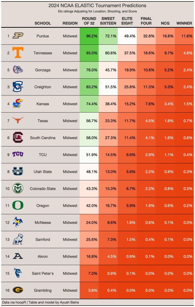
In the Midwest, Purdue and Tennessee are the most likely to make the Final Four. In this region, Gonzaga is a strong 5 seed (ranked 11th in ELASTIC), so the ELASTIC ratings do not see a strong chance of McNeese upsetting them. Kansas is a solid favorite against Samford according to these results, but it is important to note that ELASTIC does not take injuries into account so in reality Kansas is less likely to win than shown. The injury to Kevin McCullar combined with Kansas’s limited depth make Samford over Kansas a possible upset in the first round. Even though ELASTIC likes South Carolina compared to other metrics, it still has South Carolina as a weak 6 seed that is vulnerable to being upset by 11 seed Oregon.
Final Four

The most likely Final Four according to these predictions is UConn, Arizona, Houston, and Purdue. Of course, there will likely be 1 or 2 surprise teams that were not expected to make the Final Four at all, as there are in most years. Some teams that are stronger than their seed suggests (and could make a deep run) are Auburn, Gonzaga, and New Mexico. Teams that are weaker than their seed suggests (and could be upset early on) include North Carolina, Marquette, Kentucky, and Kansas. Even though March Madness is fun because of all the unpredictable upsets, it is usually the case that one of the best teams from the season ultimately wins the championship. UConn, Houston, Purdue, Auburn, and Iowa State have the best chance of winning the national championship.
